Abstract The problem of optimizing certain polar convex regions has been a topic left unaddressed for many years. Recently, many beautiful results have been obtained related to prepositions invoked in conceptual spaces. Problems currently under investigation include verifying whether the notion of polar convexity extends to plural landmarks (see Mador-Haim and Winter, 2015).
Based on the work of Zwarts and Gardenfors (Journal of Logic, Language and Information. 25, 109–138, 2016), we introduce and study optimization problems over polar convex regions and propose solutions by graphical methods. Through an interpretation of the graphical method of linear optimization, we apply this method to that of polar convex regions.
In this paper, we address the problem of polar convexity in optimization. The focus is particularly on polarizing the graphical method from its linear applications. We further discuss whether polar convexity is a necessary condition for polar optimization to remain feasible. Our results generalize previous studies that conclude certain regions are polar convex when analyzing polar coordinates as opposed to Cartesian coordinates (Zwarts and Gardenfors). In the next section, an overview of the classical graphical method for linear optimization is provided. Through graphed examples, we show the process of solving a maximization problem in this manner. Section 3 goes in depth regarding polar convexity and its various properties. Several key traits are defined in this section and subsequently utilized in Section 4. In Section 4, we introduce optimization problems over these previously introduced polar convex regions by illustrating solutions to the graphical method. We then introduce similar optimization problems that incorporate more complex figures. These figures may not necessarily prove to be solvable using the linear method of optimization, and as such require the newly introduced graphical method. The mentioned solutions involve polarizing the method of polarly linear optimization and polarizing interior-point methods for otherwise nonlinear optimization problems. Lastly, we conclude our thoughts on the findings discussed, as well as examine opportunities for future work. See the Appendix for subject material related to the main ideas prevailing in this paper.
We will now discuss the graphical method for linear optimization before exploring its further applications to polar convex optimization. The treatment here further generalizes that of Reeb and Leavengood; see [3] for more details. Linear optimization refers to the method of extracting one or more best outcomes from linear relationships. The optimized outcome is in general a maximization or minimization of the given linear representation. These representations possess certain limitations that inhibit their ability to reach values above or below specified thresholds. This event is also referred to as the constraint set, and it is what enacts linear programming; it is necessary to consider ongoing constraints in order to optimize results. A lower bound of zero is observed by default for all variables in the constraint set, thus avoiding negative resources. Linear inequalities are utilized to express the allotment of resources for each constraint. To maximize or minimize a linear function requires a predetermined objective function. Linear optimization maintains that an objective function can possess only first degree polynomial terms, such as 400x or 77y. The technique seeks to solve problems involving lines or planes with a constraint set of linearly related equations.
Linear optimization problems in general are expressed in terms of matrix form. There are multiple differing representations for linear programming, each with their own unique benefit. We will take a look at the methods relevant to our study here. Consider first the following representation, such that c, A, and b are matrices, x is the unknown variable involved in the constraint set and objective function, and each value is real and continuous:

This generalization can be referred to as the standard form. Values c, b, and x are to be viewed conceptually as column vectors, while A is an m x n matrix such that the element in row i, column j is Aij. In addition, cTx denotes the transpose of the c vector, in terms of its usual definition. Notice too that the value of x is non-negative. This holds true for all values considered in the standard form, since we seek to avoid the expression of negative resources. Moreover, the optimization type is a maximization, which remains the case in all standard form examples. To be a viable representation of standard form, a linear program must be a maximization problem involving strictly non-negative variables, where only equality statements are utilized to express relationships between variables. We can further express problems involving minimization or linear inequalities in terms of maximization and thus the standard form. In fact, all linear optimization problems can be adjusted and formatted into the standard form.
Example 2.1 Consider example 2.1, where we take a collection of linear inequality constraints and turn them into statements of equality. In doing so, the given minimization problem is manipulated into an eligible standard form maximization problem. As before, x1, x2, and x3 are real, continuous values such that the following quantities hold true.

To organize this into the standard form, we must alter the linear inequalities beneath the objective function into respective statements of equality. We also have to express the linear program in terms of a maximization as opposed to the current minimization approach. This can be achieved by applying the algorithm max = -min, which entails taking the opposite of each element of the objective function. Let z = 4x1 + 5x2 - x3. Then, max=z’ such that z’ = -z. Hence, z’ = −4x1 - 5x2 + x3. Next, we rearrange the inequality constraints into statements of equality. This is made possible by introducing either a slack or surplus variable. A slack variable is a non-negative real valued variable used in the less than or equal to case. It is added onto the remaining variables in the inequality. In an analogous way, a surplus variable is a non-negative real valued variable used in the greater than or equal to case. It is subtracted off of the remaining variables in the inequality. In example 2, it is evident that we need a surplus variable in the line −x1 + x2 + 4x3 ≥ 18, and we also need a slack variable in the line −2x1 + 3x2 + x3 ≤ 5. Let x4 and x5 represent decision variables, such that x4 is a slack variable and x5 is a surplus variable. Then, the new linear equality statements are as follows: −x1 + x2 + 4x3 - x5 = 18 and −2x1 + 3x2 + x3 + x4 = 5. x1 + 7x2 - 2x3 = 1 remains unchanged, since it already possesses the desired equals sign. As such, the following representation is logically equivalent to Example 2.1:

Another form worth noting is canonical form. It follows a similar structure to standard form linear programs, with a certain key difference. The canonical form is able to be expressed in terms of a linear inequality constraint, while the standard form requires the constraint set to involve strictly statements of equality. The two forms are similar, though, in that both require non-negativity among decision variables, along with containing objective functions that maximize parameters. Here is the canonical form of a linear optimization problem:

To convert from one form to the other requires a transformation using matrices and column vectors. In order to go from standard form to canonical form, one must replace A and b in Ax = b, such that the new representation is Ax ≤ b. In canonical form, A is of the matrix form: [A −A]. Similarly, b is of the column vector form as follows: [-b b].
Next, we will take a look at the process of graphically solving a linear optimization problem. We have already observed the first step, which is to translate an appropriate problem into its resulting objective function and list of constraint inequalities. We now show the remaining process for solving problems involving linear programming.
Example 2.2 Consider the following example, 2.2, which illustrates a maximization problem involving two constraint inequalities. All values are restricted to be non-negative. Note that since there are only two variables, we can solve this problem graphically in two dimensions. If there exists n variables, such that n ≥ 1, then the resulting graphed solution must be in n dimensions.
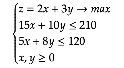
To plot the graph, we begin by rewriting the two constraint inequalities as statements of equality. Then, solve each equation for its x and y intercepts.

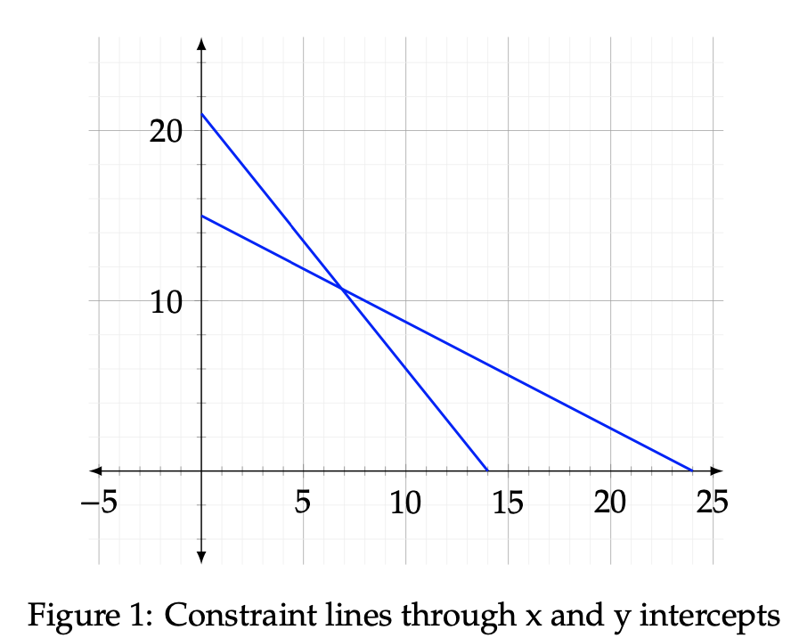
Hence, we have the following x-intercepts: (14, 0), (24, 0) and y-intercepts: (0, 21), (0, 15). We now plot the two lines in Figure 1 below containing intercepts from their corresponding constraint equations.
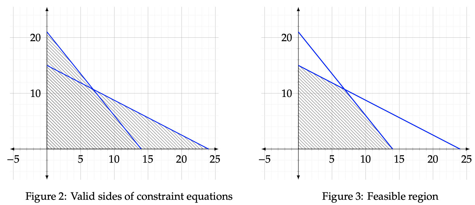
Upon displaying the two constraint lines, we then need to verify the valid side of each one. To do this, consider an example point such as the origin, (0,0), and substitute it into each constraint equation. Since 15(0) + 10(0) ≤ 210 and 5(0) + 8(0) ≤ 120, the side of each constraint line facing the origin represents the valid region. Each valid side is shaded gray below in Figure 2, with the one from 15x + 10y ≤ 210 highlighted in red and the one from 5x + 8y ≤ 120 highlighted in blue. The purpose of this step is to allow for a seamless location of the feasible region. The feasible region is the area in which the intersection of both valid sides lies. Any point that dwells outside of the valid region of a constraint line is infeasible. The feasible region is limited to strictly positive values in quadrant I due to the non-negative conditions imposed on the input variables. Below, the feasible region has been shaded in Figure 3. Notice how it ignores the portions of the previous graph that extend beyond the validity of 5x + 8y ≤ 120.
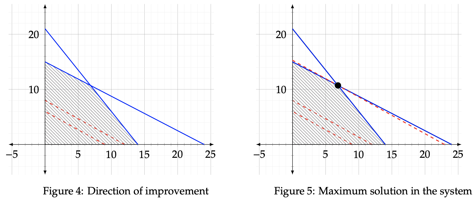
We have now established the feasible region, which means that the optimal solutions lies somewhere within the shaded region. We must determine where that point is, though, by observing the direction of improvement. The direction of improvement is meant to illustrate which way is trending toward optimization. For instance, the origin could be optimal, in which case the direction of improvement would be toward (0, 0). Alternatively, the direction could be pointed away from the origin to some undetermined point of intersection. Consider the following example in which we further display this concept. To do so, let z be equal to two arbitrary values, z = 24 and z= 18. We will then plot two objective function lines in order to verify which direction causeszto increase toward maximization. Follow the same steps as before to isolate the x and y intercepts as follows:

Now observe these two lines plotted with their respective intercepts alongside the previous feasible region graph we ascertained. The direction of improvement lines are displayed in the Figure 4 below. As the plotted lines move away from the origin, the value of z increases, since the blue line corresponds to z = 24 and the red line corresponds to z = 18. Hence, we can conclude that the maximum value of z lies in the direction away from the origin. The exact maximum value of the optimization problem occurs at the point furthest away from the origin, whilst still maintaining a presence in the feasible region. That point has been bolded in Figure 5. Notice that it dwells at the intersection of the two constraint equations.
Now that the maximization point has been spotted, we can solve for it by setting up a system of two equations. The solution (x,y) will then represent the maximal output given the constraints.
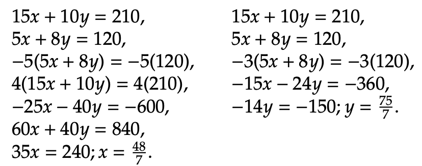
Hence, the optimal solution is at (48/7, 75/7). To determine the maximum z value for the objective function, we input x = 48/7 and y = 75/7 into z = 2x + 3y. Therefore, z = 2(48/7) + 3(75/7) = 7. We can conclude that the maximum value of z, given the two constraint inequalities, is 321/7.
There are several other constraint types that pertain to various linear programming problems. One is known as the mixture constraint, and it occurs when a constraint equation passes through the origin (0,0). Another way to conceptualize mixture constraints is to think of one quantity being limited to a certain frequency based on another quantity. Two or more variables are strictly related amid this constraint type.
An alternative constraint type is the equality constraint. This type of constraint is analagous to the mixture constraint, except it combines two or more variables alongside coefficients to form a statement of equality. This leads to the removal of a valid side, as we expressed before, and instead allows for solutions that lie strictly on its line.
At other times, we may experience optimization problems with multiple optimal solutions. This occurs when the problem includes a larger assortment of constraint inequalities instead of two. There are then more possible maximization points in the feasible region, which each correspond to a specific z output. The largest z value represents the maximum solution, and z is not limited to one point. For instance, if two points in the feasible region each correlate with the same maximum output value, then that optimization problem contains two unique solutions.
Unbounded solutions also come into consideration in some applications. These occur when one is provided with an unlimited allotment of resources, and the challenge is then to provide further constraints that may have been overlooked. Without additional constraint inequalities, the linear programming problem will not make logical sense. For example, consider the constraint equation y = 10. If we were to graph that constraint on the above coordinate planes, it would originate from (0, 10) due to the non-negativity condition for x and y. The plotted line would then proceed to the right for an infinite length of time, and thus we could improve the solution infinitely by continually adding more of the y resource. Adding one or more subsequent constraints will allow us to pinpoint an exact solution that makes sense within the confines of linear optimization.
We will now discuss p-convex sets before exploring their parallels with the graphical method for linear optimization. We then move toward our proposition of a new method, the graphical method for p-convex optimization. The treatment here generalizes that of Zwarts and Gardenfors; see [1] for further details. To begin talking about p-convex sets, let us first consider the notion of convexity. A subset C is referred to as convex if all points that lie between x, y ∈ C are also in C. The word between can be thought of as a relation between a trajector and two or more landmarks, in this case x and y. There are a variety of other ways to frame the concept of betweenness. We will deploy one below, which demonstrates the principle from Euclidean geometry that points between x and y in C reside on a line between x and y. Consider Figure 6, which include one convex region and another region that withholds convexity.
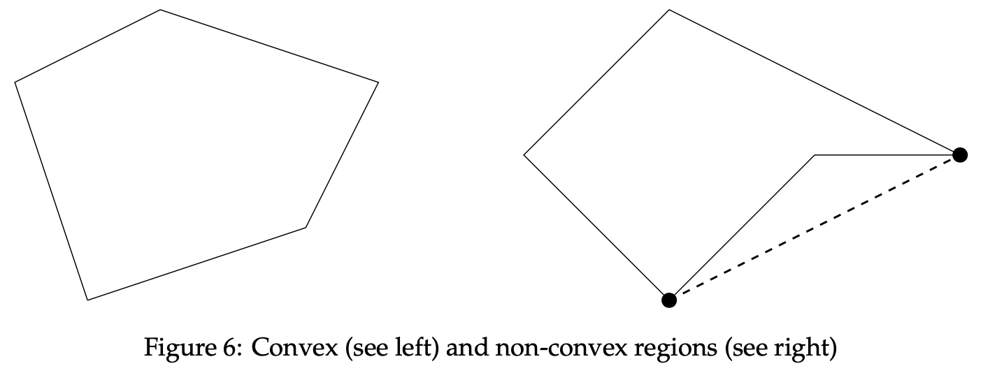
For a region to be convex, each point dwelling between points x and y must also be in the figure C. In the above examples, C can be represented by the two distinct shapes inside the boundary lines. Now take a look at the dashed line between the two marked points. This line possesses points between the two bold dots, x and y, that lie outside of C. Therefore, the rightmost figure is not convex. In the left shape, any two points can be selected within C that maintain the property of betweenness. Hence, we conclude that this region is convex.
We can also introduce the idea of open and closed convex sets. To define these two entities, first examine the concept of extreme points. Let C be a convex set. Then, a point x ∈ C is an extreme point iff there does not exist direction vector D such that D and -D are feasible directions at x. Using this definition, we can further assert open and closed convex sets as follows: An open convex set is a type of convex set that has no extreme points. A closed convex set is the complement of an open convex set, and contains strictly extreme bordering points. Consider the following examples in Figure 7, each of which express different properties of convexity that we just discussed.

The leftmost figure is a closed convex set. It has extreme points and no gaps around its bordering edges. Conversely, the middle figure is an open convex set. While it still passes the betweenness checks we performed above (in fact, both figures from the previous example would be considered open, with the one on the left convex and the other not convex), it does not have any extreme points. Therefore, it is open and convex. On the right, we can see that the region contains gaps among its extreme points. This assuredly means it is not a closed convex set. However, it still holds for extreme points, and as such is not open convex either. Hence, the rightmost figure is neither open convex nor closed convex.
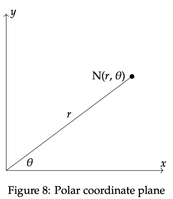
It is possible to further extend this concept of betweenness to the 3-dimensional Cartesian, spherical, and cylindrical coordinate planes. For our purposes, we will place emphasis on polar coordinates in two dimensions, hereby expressing another notion of betweenness involving polar convexity. See the Appendix for further information regarding multi-dimensional coordinate systems for convexity. In two dimensions, polar coordinates can be thought of as an alternative way to plot and represent space. They illustrate points in terms of their respective distance and angles as opposed to the Cartesian (x, y) plane. Using polar coordinates, a point in the plane is determined by its angle, θ, and its distance from the origin, r. The angle theta lies strictly between the x-axis and the radius line. See Figure 8 below for an example graph using polar coordinates and the point N = (r, θ):
The polar representation of a point in a plane, such as the one provided above, has an accompanying visual interpretation as well. We investigate this approach now in order to provide a more simplistic and comprehensible approach to the graphical method subsequently. The following polar coordinate system particularly contains the radius, r, as the directed distance between a point and the origin. The angle between the point and the x-axis, θ, will then be incorporated in a full circle around the graph. Positive angles are included in a counterclockwise direction, while negative angles are measured clockwise. In the next graph, we look to represent the example point (r, θ) = (6, π):
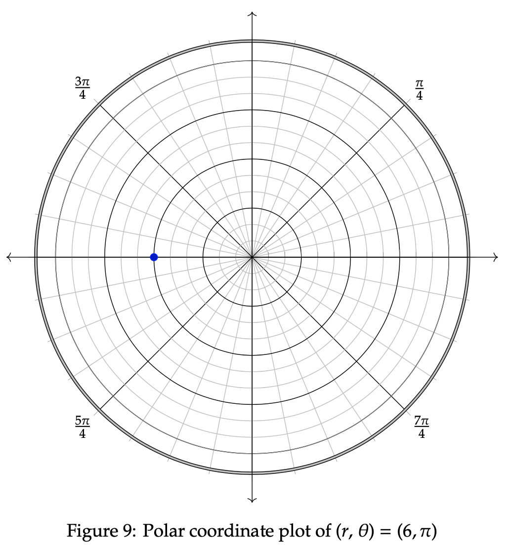
The line segment extending rightward from the center point is called the polar axis. In terms of Cartesian coordinates, this would be known as the x-axis. The center point is referred to as the pole, and correlates to a radius of r = 0. The point plotted above rests 6 units from the pole. Since 6 is a positive value, we measure θ = π starting from the polar axis and continuing counterclockwise until we reach the location where π resides on the circle. This process is followed when plotting any point or figure on the polar graph.
To move forward in our discussion of polar convexity, we must first establish the concept of polar betweenness. We have already gained insight into the Cartesian conviction of ”between.” However, the polar between definition and consequences differ in key instances. Consider the following definition for polar betweenness, assuming that we are presented with a valid representation of polar coordinates as defined above:

Polar betweenness is undefined when |θa - θb| = 180º. Additionally, when A or B is at the origin point, we can set θa = θb, since values of θ are undefined in this case. Now possessing the intuition behind polar betweenness, we can look at two distinct examples, the first of which displays polar between points and the second does not.
Example 3.1 Consider Example 3.1, where three points are plotted below in the polar graph. We wish to show that the middle point, (6, π), is polar between (12, π) and (3, π), which are the red and brown points, respectively. To verify that these points display polar betweenness, we must show that there exists an integer k from 0 < k < 1 such that the above equations hold true.
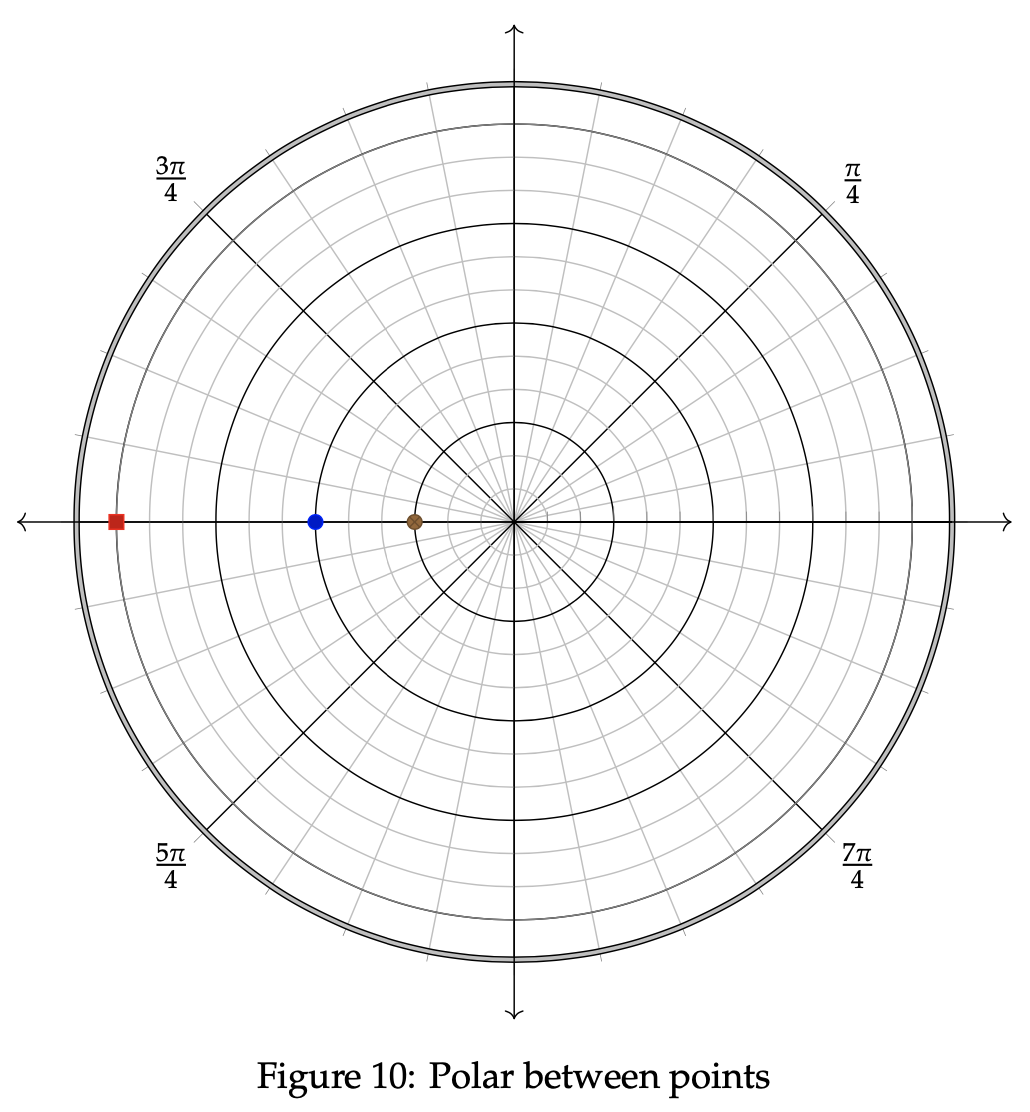
Let us first examine the radius equality property using the provided equations. We know that rn = 6, ra = 12, and rb = 3, so the following simplification extends from that:

Therefore, the definition of polar between holds for the radius equation. Next, we show that it holds for the angular equation as well. We know that θn = π, θa =π, and θb = π. Since |π - π| = 0 < π, the first equation for theta is applied:

In this case, any value of k between 0 and 1 satisfies the condition for polar betweenness. As such, we can conclude the blue point is polar between the red and brown points.
Example 3.2 Let us now examine three points that do not display the property of polar betweenness. Consider Example 3.2, which again possesses three coordinate points within its axes. We wish to show that the middle point, (6, π), is not polar between (9, 3π/4) and (12, 5π/4), which are the red and brown points, respectively.
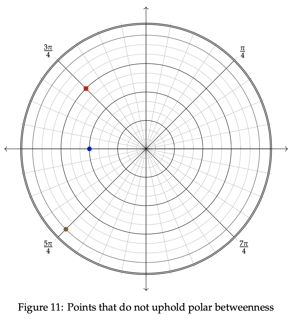
We again check to see if the blue point is polar between the other two, using the defined formulas. First, we check to see if the radius equation holds true. It is known that rn = 6, ra = 9, and rb = 12, so the following simplification extends from that:
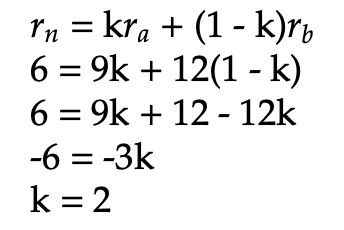
Therefore, the definition of polar between does not hold for the radius equation because k = 2 exceeds the range of possible values for k. Hence, it is unnecessary to attempt to show that the graph holds for the angular equation, since it already fails for the radius. We can thus conclude that the blue point is not polar between the red and brown points in this example.
With this definition now invoked, we can define the property of polar convexity. The concept follows similarly to that of Cartesian convexity, except translated into the polar coordinate system. Consider the following formal definition for polar convexity, before taking a look at a few examples of figures that express the property.
Let R be a subset of a conceptual space S. Then, R is polar convex if and only if for all points a and b in R, any point N that exists in S that is polar between a and b is also in R.
This extends in a similar manner to the polar between points we analyzed previously. This time, though, there will be a region R containing "red" and ”brown” points. If every possible ”blue” point that is polar between the red and brown ones lies within R, then R is polar convex. Several key figures are polar convex, such as a sphere, a plane, an infinite cone, a half-space, a half-plane, and a line. This is not an exhaustive list of such regions, and simply represents a small sample of eligible figures. Let us now consider a circle, which is an example of a polar convex figure.
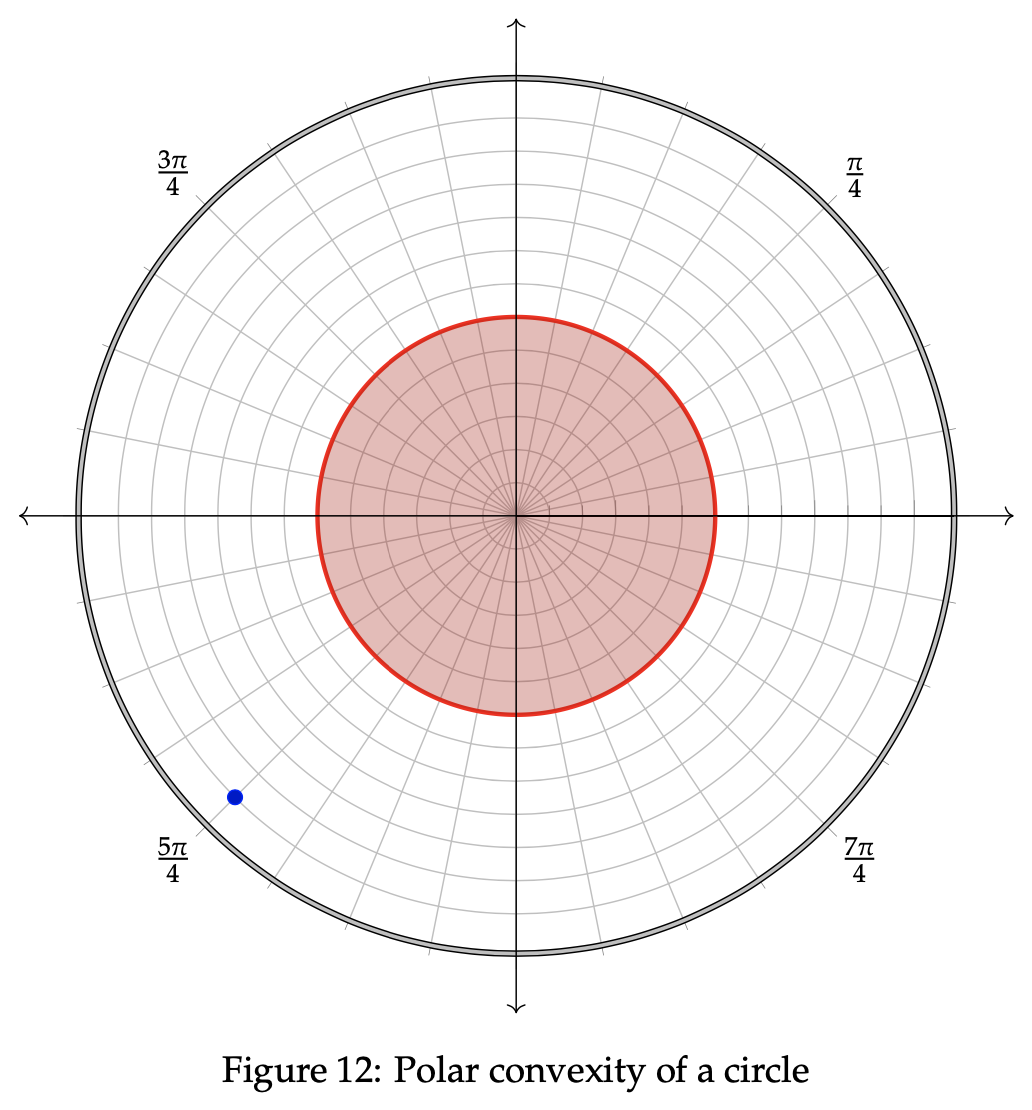
Take a look at the plotted points in the above circle. We can see that for any two points a and b in the circular region, R, any point polar between the two points also lies within R. The blue point in this case neither lies in R nor lies polar between any two points a and b, so it does not preclude R from exhibiting polar convexity. Therefore, we can necessitate that both a and b must be chosen strictly from the figure R, as specified in the definition.
We can also discuss the polar convexity properties of the intersection between regions. If two regions are polar convex and centered around the same distinct point, then their intersection is polar convex as well. This property becomes increasingly useful when dealing with pairs or conglomerations of figures.
Conversely, there are specific regions for which polar convexity does not hold. Consider a region R such that R is a subset of the conceptual space S. Given two points x, y ∈ R, if we can locate a point that is polar between the two points and outside of the region R, then R is not polar convex. This is similar to the latter half of the first example in section 3, except translated to polar coordinates as opposed to Cartesian coordinates. Some example figures that do not fall under the realm of polar convexity are triangles, cylinders, double cones, and cubes. Look below at Example 3.3 for closer insight into what disqualifies a figure from polar convexity.
Example 3.3 In this example, we will take a closer look at a polar square figure. We wish to show that the square region, R, does not display polar convexity. In order to show this property, two points will need to be located within R that contain one common point polar between point them that is outside of R.
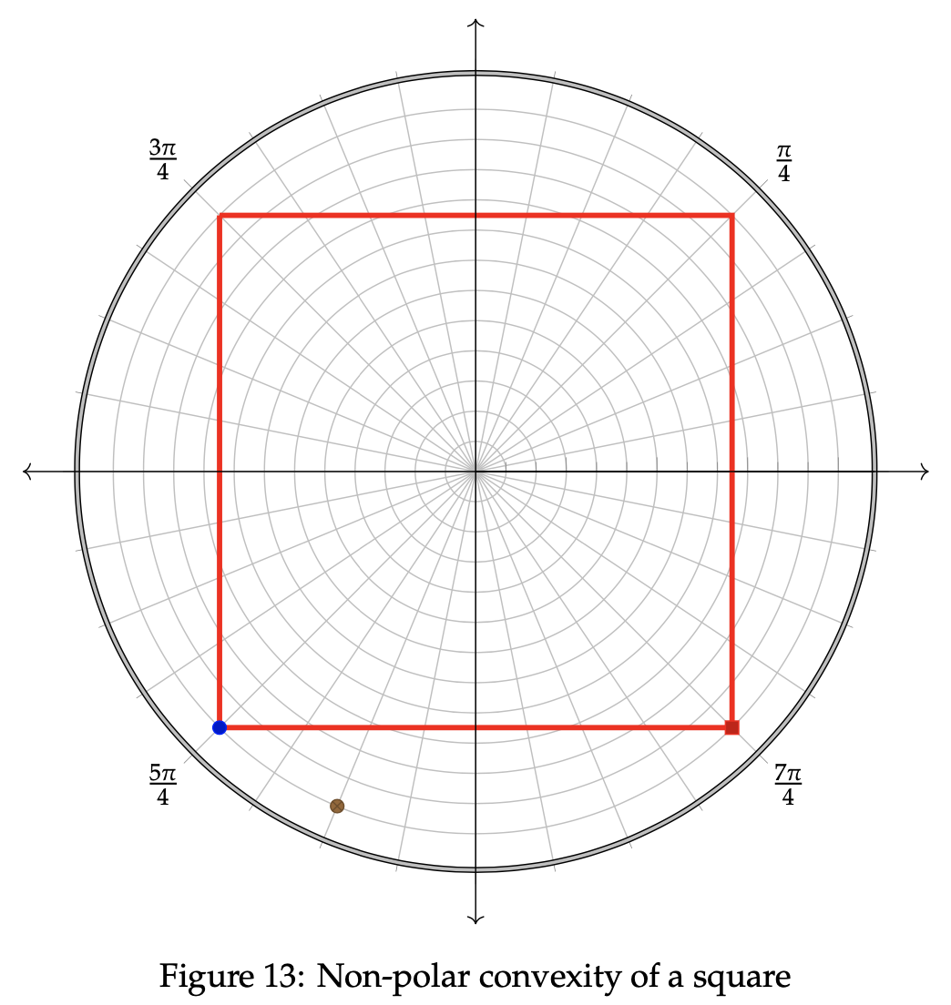
Let the blue point above represent a and the red point represent b in the definition of polar convexity. Now, in order for the region to hold for non-polar convexity, we must locate a point N such that N is polar between a and b and lies outside of R. Let the brown point represent N in this case. We wish to show that N is polar between a and b. Proceed again by using the definition of polar betweenness. To verify that these points display polar betweenness, we must show that there exists an integer k from 0 < k < 1 such that the polar between equations hold true. Let us first examine the radius equality. We know that rn = 11, ra = 11, and rb = 11, so the following simplification extends from that:
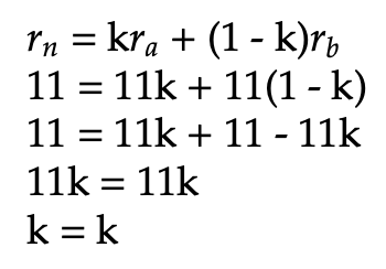
We can utilize any value for k between 0 and 1 to fulfill the pre-condition for k. Therefore, the definition of polar between holds for the radius equation. Next, we show that it holds for the angular equation as well. We know that θn = 11π/8, θa = 5π/4, and θb = 7π/4. Since |5π/4 - 7π/4| = π/2 < π, the first equation for theta is applied:
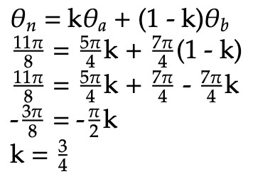
Since the k value falls between 0 and 1, we can conclude that N is polar between a and b. However, N is not contained within R. Thus, the region R is not polar convex, as desired.
In the next section, we seek to optimize the types of polarly convex figures encountered in the example involving a circle. Adapting the graphical method for linear optimization to fit polar regions will help in our efforts to do so.
In this section, we propose a new method for graphically analyzing p-convex optimization. The concept is formulated compoundly using the topics of polar convexity and the graphical method for linear optimization encountered in the previous two sections.
To begin talking about the optimization of p-convex shapes, let us first mention a pertinent example that aids in the visualization process. In this example, we possess both a spherical stone and a circular pool of water. The dimensions of the stone need not be revealed; we need only the ability to accurately throw this stone into the pool of water. Initially, we hurl the stone into the exact center of the pool. The interaction then follows the principle of minimum energy, which in this case indicates that the pool seeks a state in which its energy is minimized. In other words, ripples resonate outward from the stone, and they extend outward to the boundaries of the pool. Since the pool is circular and the stone is spherical, these ripples will reach the outer bounds at precisely the same time throughout the circumference. However, let us now repeat the throwing process with the same parameters observed, except for the landing spot of the stone. This time, the stone splashes down in the first quadrant of the pool. While the ripple process occurs in the same fashion as before, the outermost ripples will reach the bounds in the first quadrant before they reach those of the other quadrants. This is due to the changed ”origin” point of the stone and will play a key role in the method of polar convex optimization.
With that illustrative example revealed, we can next reconsider the notion of optimization discussed earlier. This necessitates an objective function as before, along with a set of constraints that the maximization or minimization is subjected to undergo. In this section, we deal with strictly polar convex regions, which differ from the intersection of lines studied in the Cartesian plane from section 2. However, note that a line segment is still polar convex if and only if it contains the origin point. This was indirectly shown in the example in section 3 where three points were plotted along the polar π axis. If we extrapolate the three points into a line segment including the origin, (0, 0), then the polar betweenness property would remain intact. Moving forward, various exemplary regions will be explored that display polar convexity.
We have the following workflow of seven steps to find the maximum or minimum value of a polar region graphically:
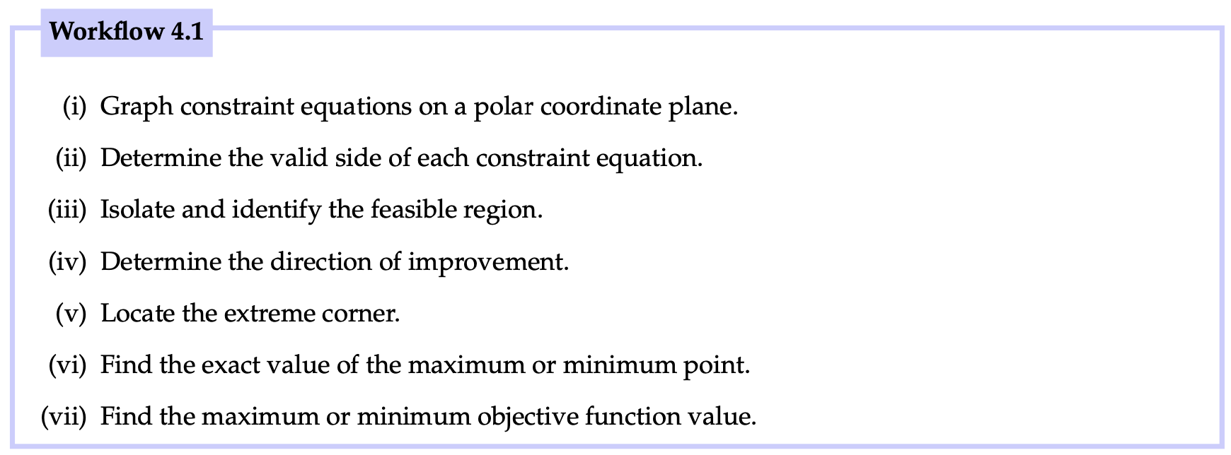
As a direct application of the above steps, we have the following examples. Each example discussed will possess a systematic approach to finding a solution that stems from the workflow above.
Example 4.1 To help illustrate the optimization process involving polar convex regions, let us consider a first example. A variant of the p-convex circle from a previous example from section 3 will be utilized. It corresponds to a maximum θ value of 2π. As in our earlier study of Cartesian optimization, all constraints are strictly non-negative values of r and θ. We wish to maximize the following objective function using the constraints listed:

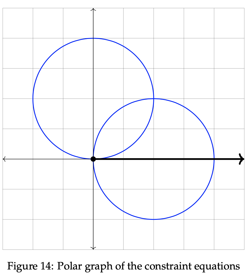
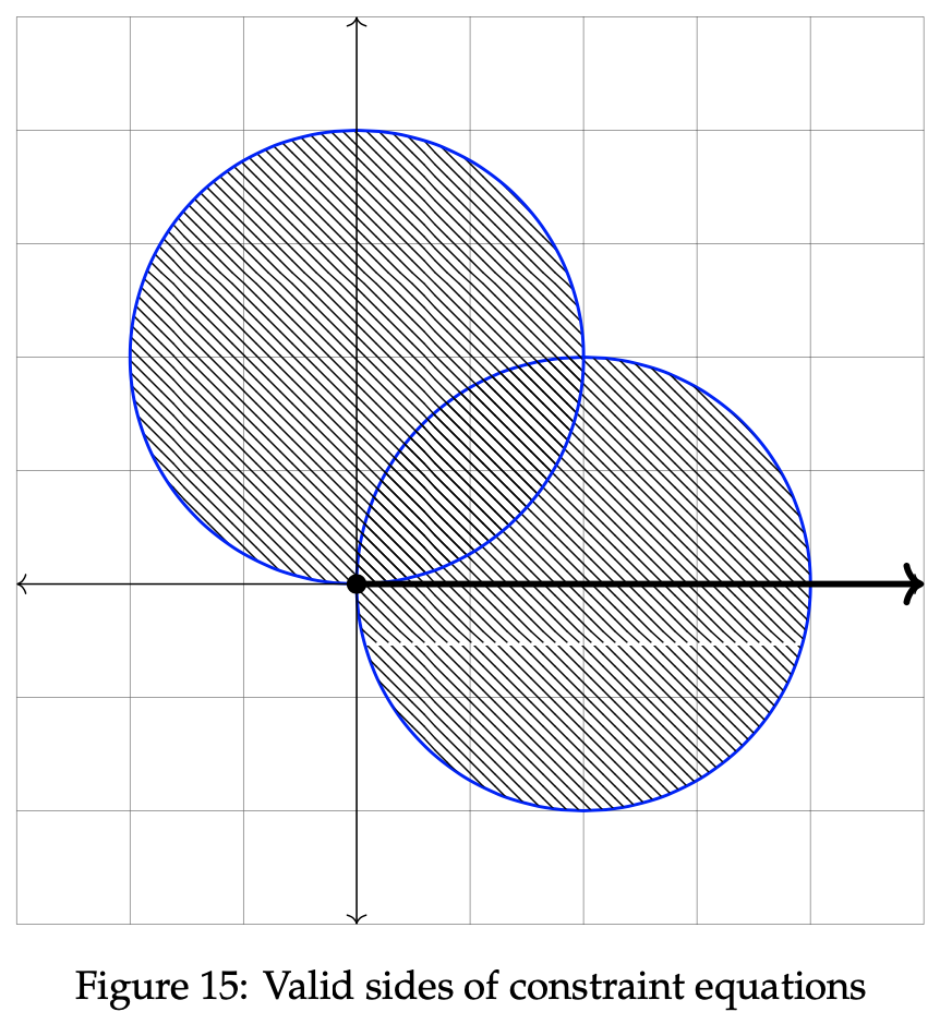
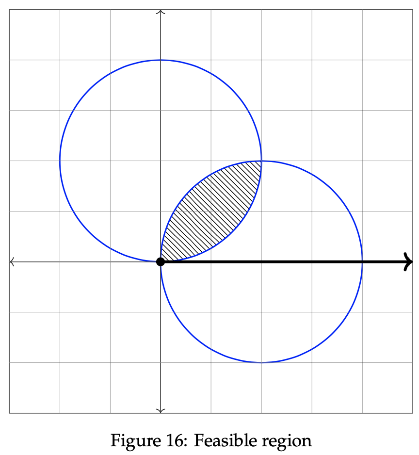
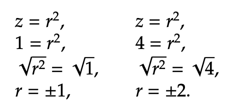
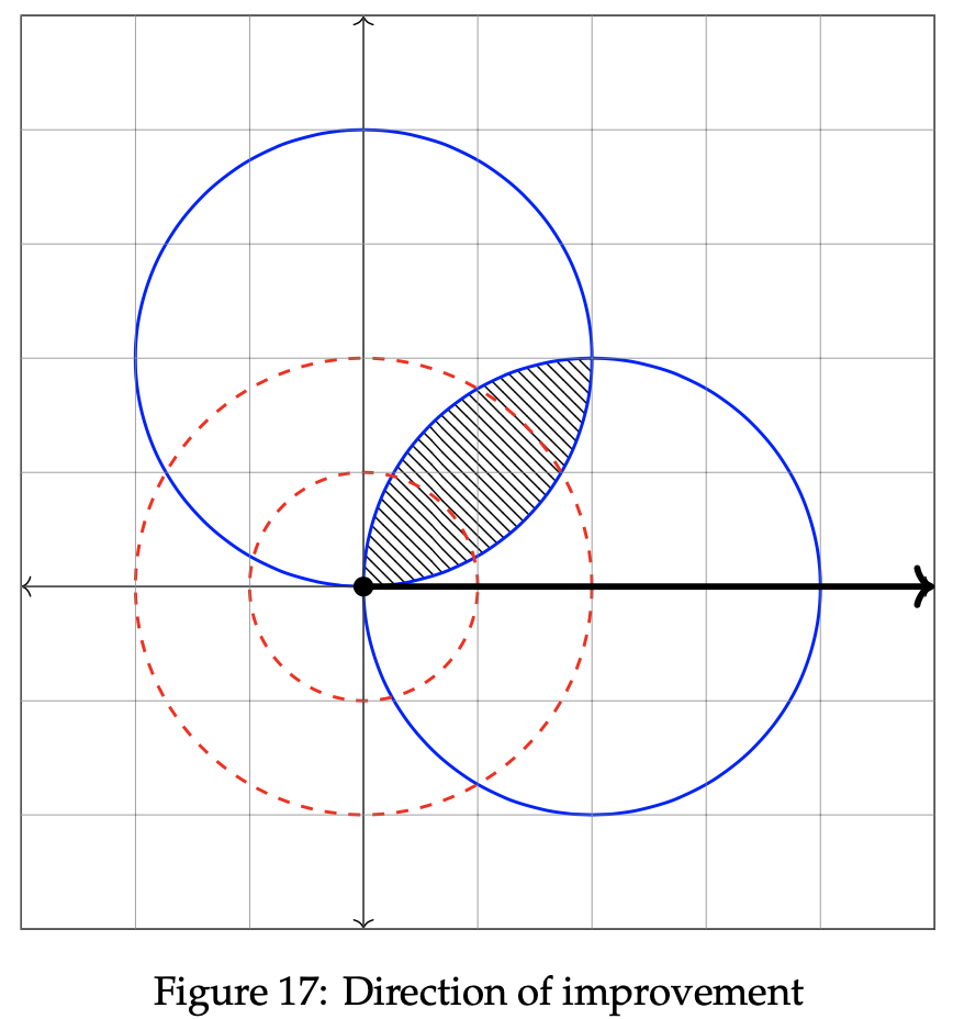
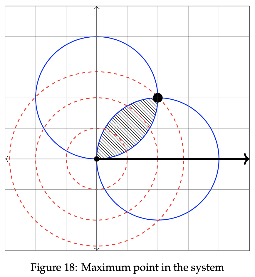
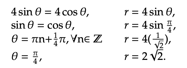
Example 4.2 Let us now consider another example involving alternative polar convex regions. A p-convex circle will still be incorporated, but this time we add a constraint line along with an objective function line as well. Recall that lines are polar convex, thus fitting with our intended focus in this study. As before, all constraints are strictly non-negative values of r and θ. We wish to maximize the following objective function using the constraints listed:

The polar graph below displays the two constraint inequalities involving r and θ. To proceed in the optimization process, the next step is to identify the valid sides of the listed constraints. As seen in the previous example, the valid side of the circle is simply each point on or within the circle itself. It is shaded in below. To find the valid side of the line, though, we must plug in a sample point to the inequality. Consider (r, θ) = (0, 0):
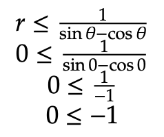
Since the final inequality is logically false, we can conclude that the valid side of the line rests opposite the side containing (0, 0). As done in section 2, the next step is completed by identifying the feasible region of the graph. Since the feasible region is simply the intersection of each valid side, the feasible region can be reduced to the location on or inside the overlap between the circle and the valid line side. We graph it below in the rightmost graph:
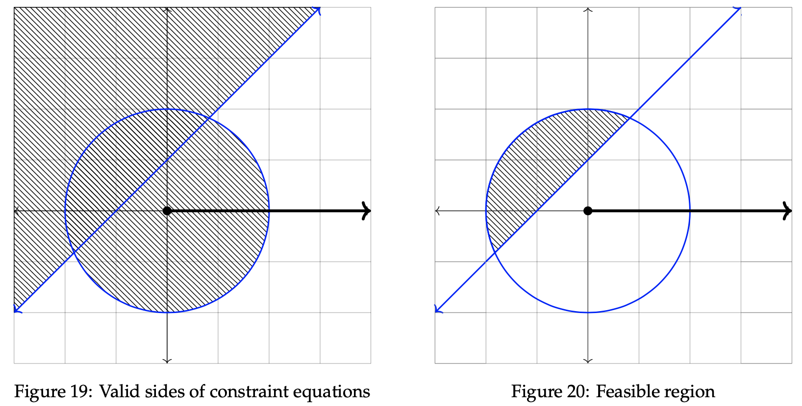
Having established the feasible region, we know that the optimal solution lies somewhere within the shaded area above. We determine where that point is by analyzing the direction of improvement. As done in example 1, we begin by selecting two arbitrary values for z. Doing so allows us to check whether larger or smaller values of z result in a maximization. Let z = −1 and z = −1/2. We will then plot two objective function lines in order to verify which direction causeszto increase toward maximization. The two lines are plotted below on the graph.
These figures inform us that as the value of z increases, the solution trends toward a maximization since the green line correlates to z = −1 and the orange line correlates to z = −1/2. Hence, we can conclude that the maximum value of z lies at the top right point within the feasible region. It is graphed below. To find the exact point of the solution, first set the two constraint equations equal to one another. Doing so will allow us to extract the locations of intersection between the blue line and the red circle. It is then possible to uncover the value of θ and use that value to determine r.

That point has been bolded in the graph below. Notice that it dwells at the intersection of the two constraint equations.
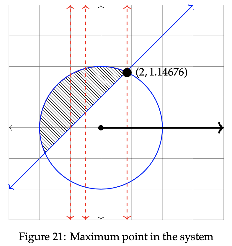
Hence, the optimal solution is at (r, θ) = (2, 1.14676). To determine the maximum z value for the objective function, we input r = 2 and θ = 1.14676 into z = r cos θ. Therefore, z = 2cos(1.14676) = 0.823. We can conclude that the maximum value of z, given the two constraint inequalities, is 0.823.
Example 4.3 Consider a third example involving a new figure called the torus. The torus is a surface that is formed by the revolution of a circle around a line in its plane. The figure possesses the properties of constant diameter without edges or vertices. For our purposes, we view the torus as a set of two-dimensional concentric circles. Tori are polar convex extending the definition giving earlier, which makes them a useful case study for our method. Here, we examine an example that incorporates the torus, a horizontal line, and an objective function parabola facing left.

The valid sides of the torus and line are shaded below in the left graph. On the right, the feasible region is shaded, which represents the area of intersection between the two shapes.
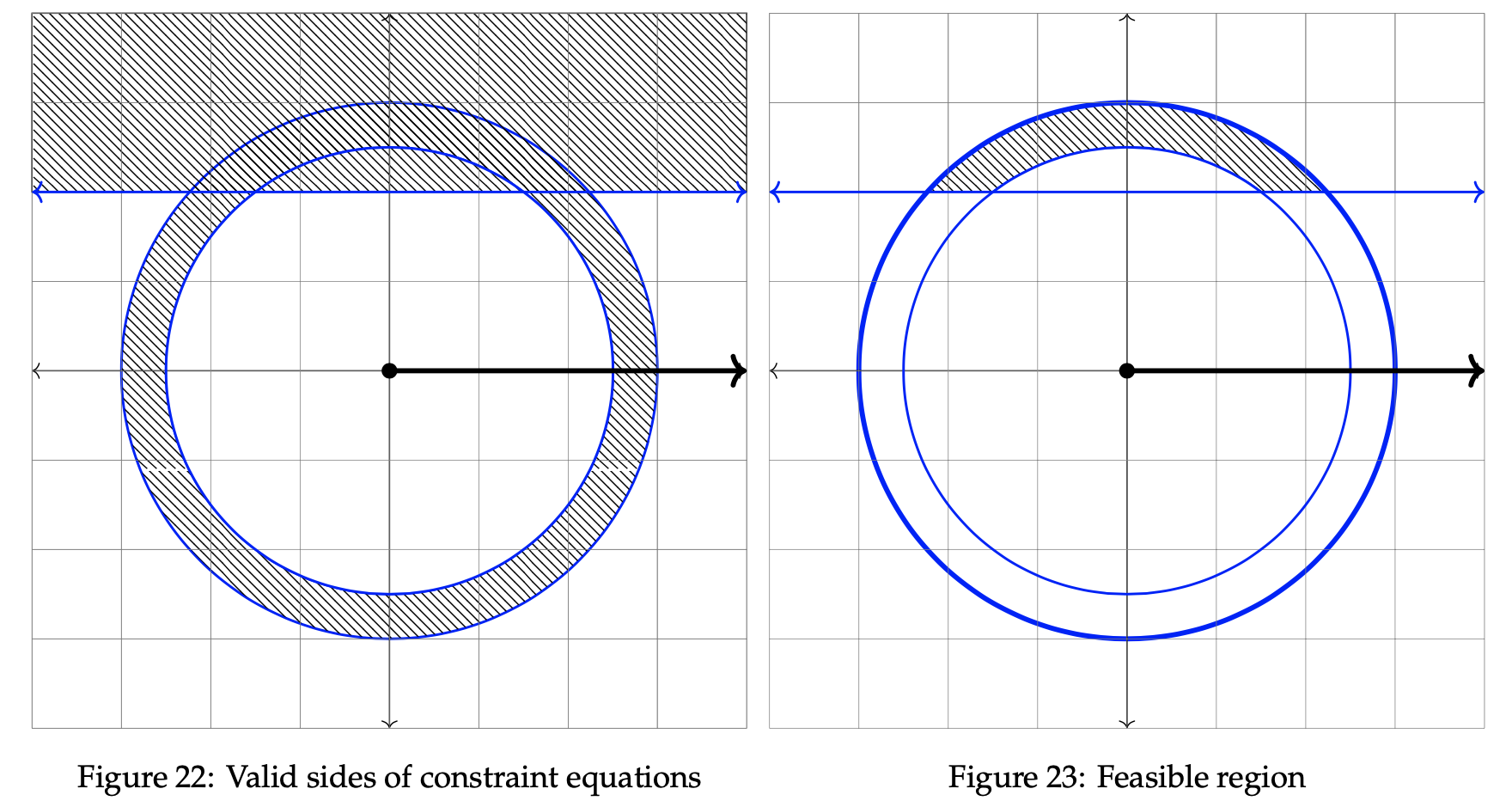
The optimal solution lies somewhere within the shaded area in the rightmost graph. Next, consider the direction of improvement. As done in the preceding examples, we select two arbitrary values for z. Let z = 1 and z = 1/2.
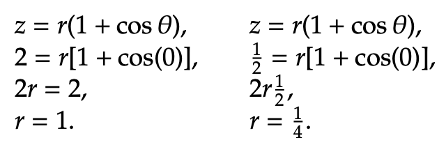
This informs us that as z increases, the problem moves toward maximization. We now plot two objective function parabolas to verify this claim. The two shapes are plotted below on the graph.
To locate the maximum value of z, we must find the rightmost point in the feasible region. To find it, set the constraint equations equal to one another to find θ. In this example, the optimal value of θ = 0.73. Then, insert that value into the line constraint equation to find r. r in this example is 3. The optimal point has been bolded in the graph below. Notice that it dwells at the intersection of the two constraint equations to the far right.
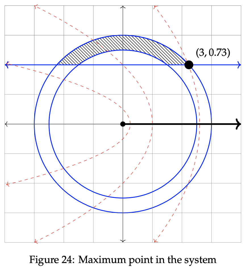
To find the exact maximum value of z, solve the objective function using the value of θ and r computed in the last step.
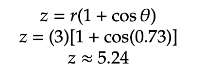
Hence, the maximum value of z in this problem is approximately 5.24.
Example 4.4 We now introduce an example involving an ellipse, another polar convex region. In this example, the ellipse interacts with a circle and line to form the feasible region. The objective function in this case is the infinity shape. It is to be maximized to fit the parameters of the ellipse, circle, and line. See below for the specific constraint equations and objective function.

In the graph below to the left, the valid sides of each constraint are shown. In the next graph on the right hand side, the intersection of these regions is shown. This intersection represents the feasible region.
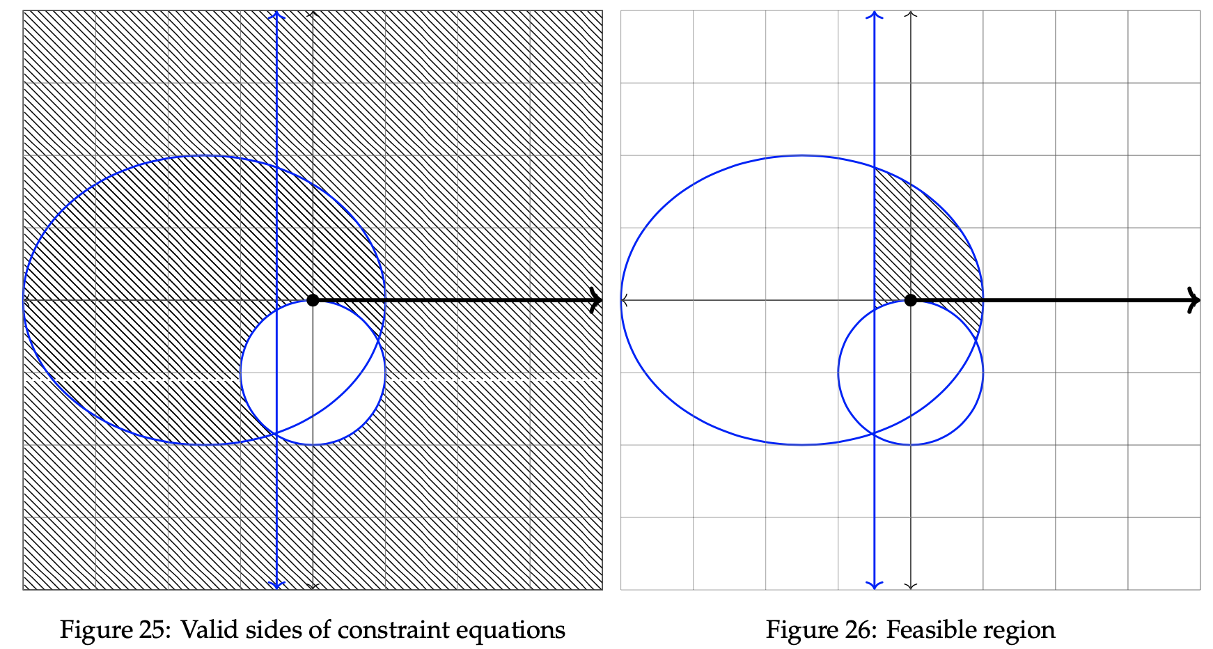
The optimal solution lies somewhere within the shaded area in the rightmost graph. As done before, we then select two arbitrary values for z. Let z = 2.25 and z = 1.
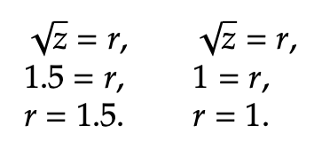
The two constraint circles are graphed below, along with the maximization point at the meeting point of the polar line and the ellipse.
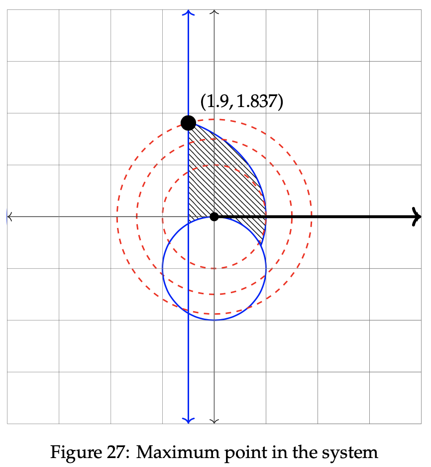
To find the actual maximization value of the objective function, insert the value of r into √z = r. We then get √z = 1.9, and z = 3.61.
Example 4.5 We now consider an example involving a minimization. Minimization problems work in a similar manner as their maximization counterparts, except for the direction of improvement step. Once there, we look for the direction that improves the least instead of the direction that improves most. This will become increasingly clear when analyzing the below example. In this example, the two lines interact with a circle to form the feasible region. The objective function in this case is a limacon, which originates from Pascal. The limacon is defined as a roulette shape formed via a fixed path of a point around a circle such that the circle rotates around the outside of another circle of equivalent radius. In this example, we find a limacon that minimizes the parameters set by the two lines and circle. See below for the specific constraint equations and objective function.

In the graphs that follow, the valid sides of each constraint are shown to the left, while the feasible region is determined and plotted in the rightmost graph. It follows from this fact that the point of minimization lies somewhere within the feasible region.
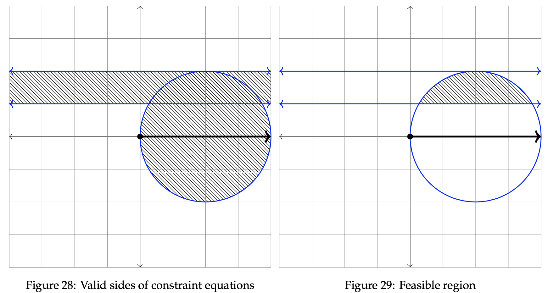
As previously done, we shade the entirety of both constraints before subsequently shading only the intersecting portions of each one. The optimal solution resides within the shaded area in Figure 29. Select two unique, arbitrary values for z to proceed in the minimization process. In this case, let z = 3 and z = 2.

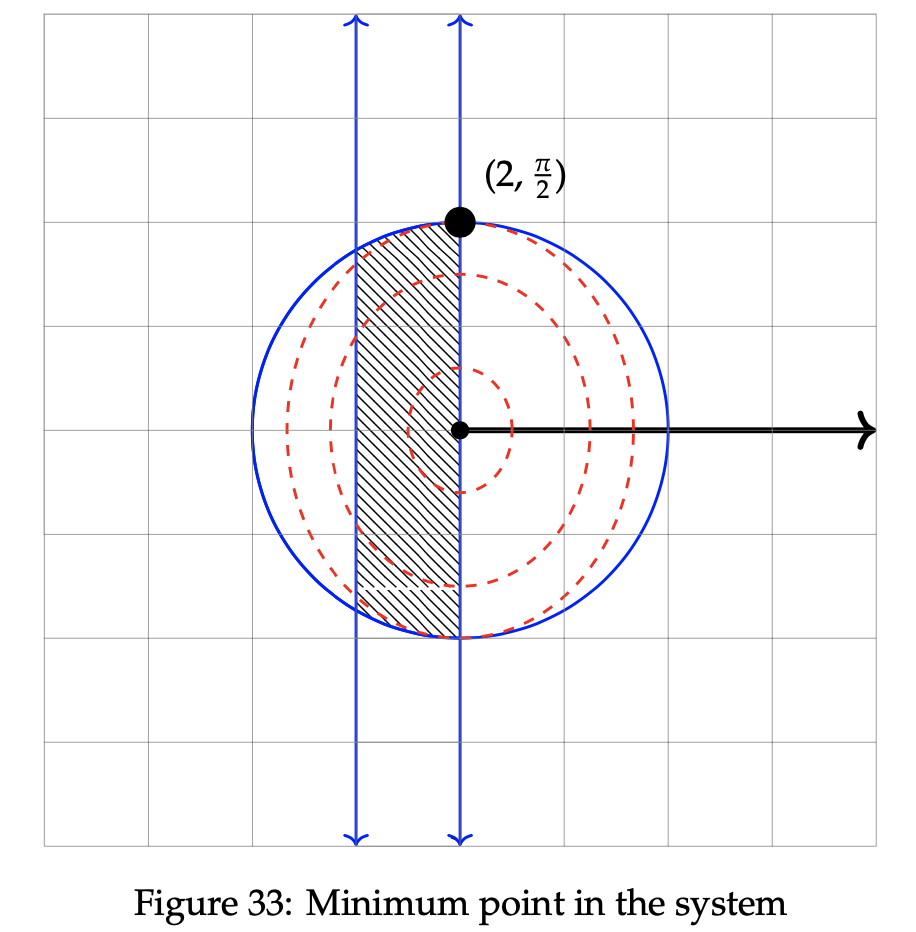
As the value of the objective function increases, θ decreases. Since we are seeking to minimize this problem, the minimum point in the system lies in the region that decreases the objective function value. In this case, that occurs when θ increases as much as possible within the confines of the feasible region. This differs from our previously encountered maximization problems, which instead seek to increase the value of the objective function and as such, choose the value of r or θ that leads to the largest value of z possible given the available constraints. It is plotted below in Figure 33.
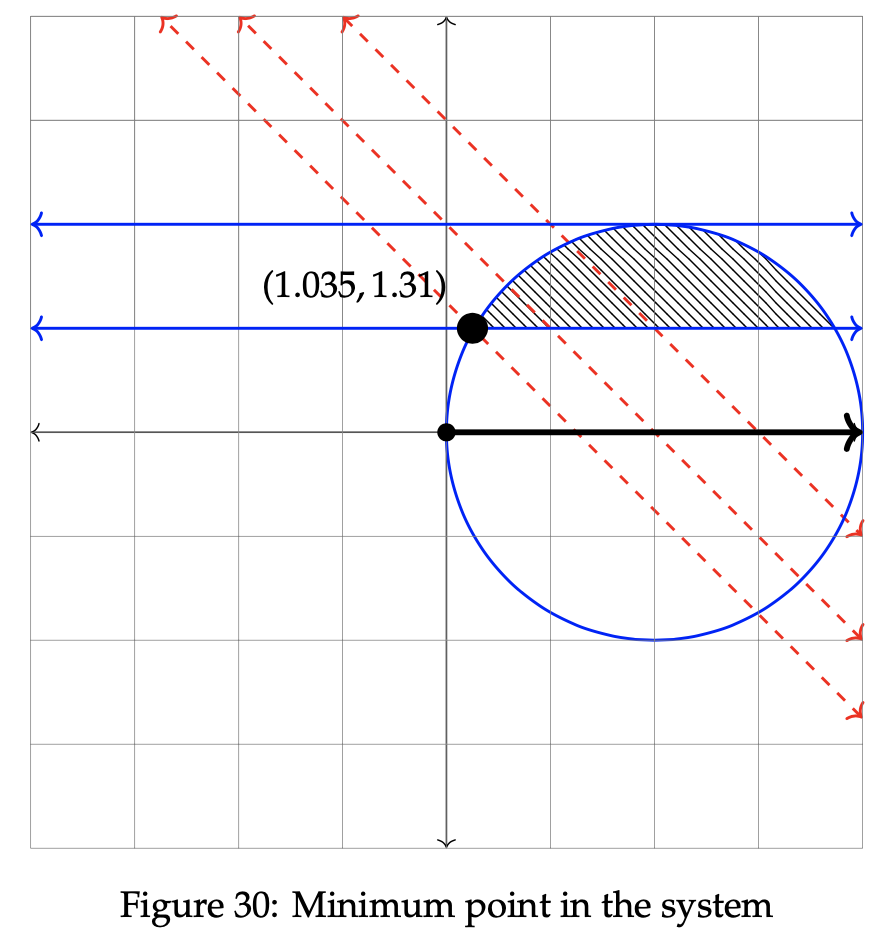
Notice in Figure 30 that the minimum point lies at the leftmost portion of the feasible region. This location corresponds to the maximum value of θ allotted within the constraint inequalities. To find the exact value of the minimized point, set the constraint equations of the circle and line equal to one another and solve for (r, θ). The result is plotted on the graph above: (r, θ) ≈ (1.035, 1.31).

Next, we illustrate the valid sides of each constraint, and also shade in the feasible region in the figures below. The maximum point resides somewhere within the feasible region.
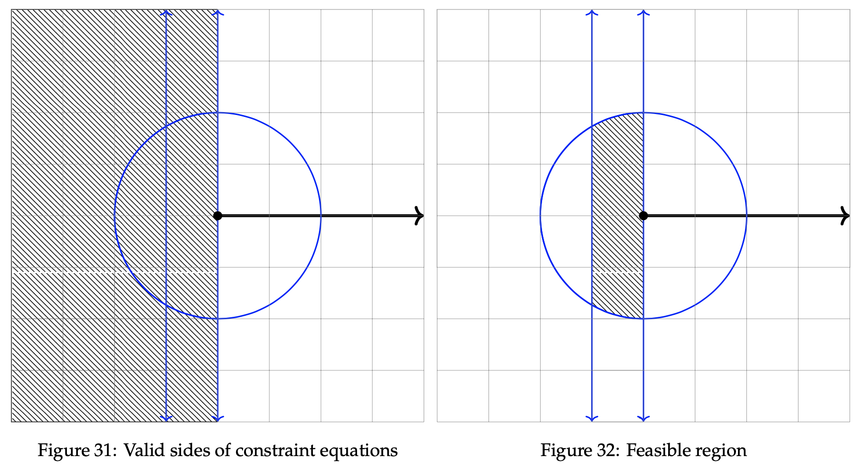
The optimal solution will be within the shaded area in Figure 32. Select two unique, arbitrary values for z to proceed in the maximization process. In this case, let z = 8 and z = 6.
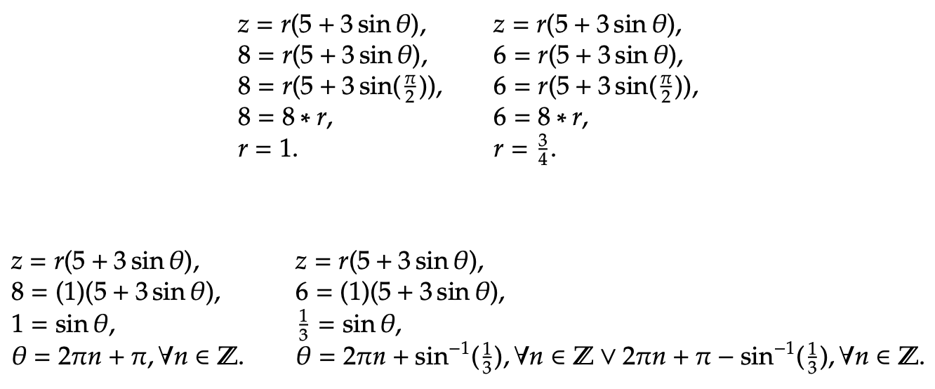
As the value of the objective function increases, r increases as well. Additionally, as z increases, θ decreases. So, our optimal point in the feasible region will be located at the intersection of the maximum radius and the minimum angle. In this case, that occurs when θ decreases as much as possible within the confines of the feasible region, to a value of π/2. The radius corresponding to this angle is r = 2, which is the largest radius possible given the constraints. The maximum point is plotted below in Figure 33, along with the objective function denoted by the dotted red ellipses.
In order to finalize our notion of polar convexity, we must consider the necessary conditions for a polar optimization problem. In the preceeding examples, we worked solely on maximizing and minimizing convex figures. Might it be possible to apply these same techniques to non-convex regions? It turns out that we cannot, as we now explore.
Earlier, a subset C was deemed convex if all points that lie between x, y ∈ C are also in C. An extension of this definition suggests that the region does not contain a local minimum or local maximum. Local extremum in this context can be viewed as “false” minimums or maximums. It does not represent the true highest or lowest point in the region, and in doing so corrupts the performance of our optimization strategy. Convex figures do not have local extremum, as they possess one distinct global minimum or global maximum. Our technique then leads to the convergence to that specific maximum or minimum, as desired.
The second derivative test can be used in polar coordinates to determine the convexity. Note that in order to do so, it is required to calculate ∂2y/∂x2 with respect to polar coordinates r and θ. Consider the following derivation of the second derivative test for polar coordinates, using the fact that x = rcos θ and y = rsin θ:

Stochastic non-linear programming is an important class of polar optimization problems that includes second-order cone linear programming and stochastic mixed-integer linear programming as special cases. In this paper, we have described six different applications that lead to polar convex optimization solutions, and this has been achieved by relaxing assumptions that include deterministic information to incorporate different examples. It is important to indicate that all of the optimization examples that have been developed in this study are intractable for an extensive form formulation.
Developing additional more specialized algorithms to solve the generic seven-stage polar optimization problem is an important subject of study. In this paper, we have commenced this study by describing solution methods for solving the generic linear optimization problem using the graphical method. We emphasize that the work presented in this paper is far from being a survey or comprehensive study, but instead that it would rather shape a basis for further research studies in polar optimization using the graphical method. In particular, it is our firm belief that this research is a rich source for stochastic models, and it can be utilized to implement numerous future algorithms for solving this class of optimization problems.
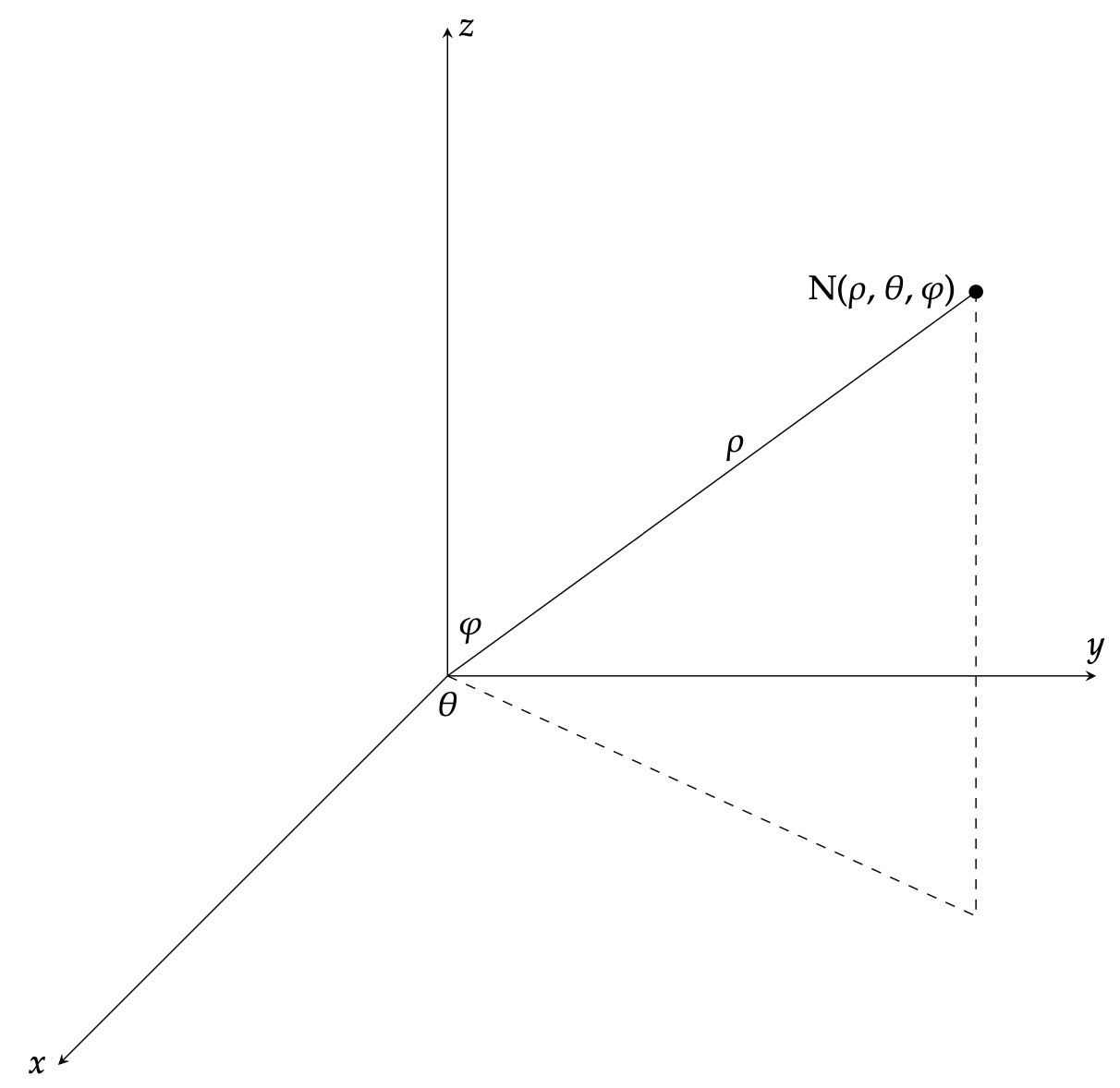
In this section, we discuss the extension of polar coordinates from two dimensions into three dimensional spherical and cylindrical coordinate systems. First, consider the following applications of spherical coordinates. Below, we define and express the three-tuple (ρ, θ, φ) in terms of the point N.
radius, ρ: a non-negative real number representing the distance between the origin point and N
azimuth angle, θ: the angle between N and the x-axis, such that 0º ≤ θ ≤ 2π
polar angle, φ: the angle between N and the z-axis, such that 0º ≤ φ ≤ π
Let us now consider how this is done in closer detail by examining an example point N in terms of its spherical coordinates. The following three-tuple (ρ, θ, φ) point will be graphed below, with definitions of ρ, θ, and φ analogous to those above. We can then derive several conversion formulas to help conceptualize spherical coordinates.
We now are able to examine some common conversion formulas that illustrate the way in which a point’s Cartesian and spherical coordinates are related. First, take a look at the converting formulas to go from spherical to Cartesian coordinates:
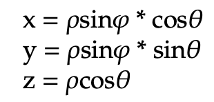
Additionally, there are formulas for the opposite relationship, converting from Cartesian coordinates to spherical coordinates:
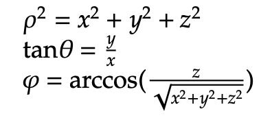
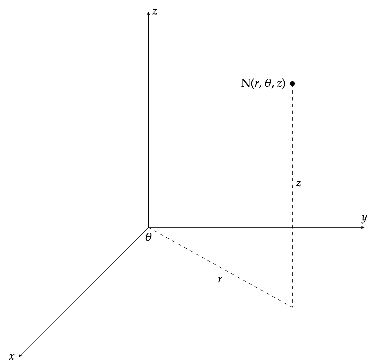
Let us now investigate cylindrical coordinates and their respective similarities and differences when compared to spherical coordinates. As before, we will end with a list of conversion formulas between the various coordinate systems. In the following representation, (r, θ) are polar coordinates of the point N’s projection in the xy-plane. z is the expected Cartesian component, which describes the location of the point as either above, on, or below the xy-plane.
Now, here are a list of conversion formulas to alter cylindrical coordinates into their Cartesian coordinate counterparts:
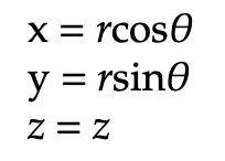
As done previously, we now express the reverse, converting from Cartesian coordinates to cylindrical coordinates. Notice the largely similar terms in each section. Additionally, keep in mind that cylindrical coordinates are simply an extension of polar coordinates with the inclusion of the z component.
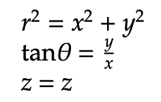
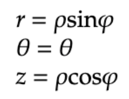
Finally, we will look at the equations used to convert from cylindrical coordinates to spherical coordinates, and vice versa. First, we examine the conversion from cylindrical to spherical:
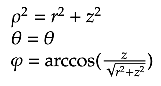
We conclude with the conversion formulas from spherical to cylindrical coordinates:
