Empirical analysis of queuing theory on transit data

Abstract The problem of analyzing transit data using queuing theory has been a topic left mostly unexplored. Recently, many useful results have been obtained related to transportation data and reduced waiting times. Problems currently under investigation include the Waiting Time Paradox [5] and applications of real-time transit data to wait times [4].

Based on the work of Liu and Miller (Transportation Research Part A, p. 167–179, 2020), we introduce and study a transportation simulation involving approximated data sets. Through an interpretation of the notion of queuing theory, we verify whether this simulation fulfills the properties of a Poisson Distribution, and if not, which distributions most accurately describe a queuing theory process with multiple queues.

Introduction

The advent and widespread use of transportation data is revolutionizing the manner in which passengers approach traveling in their daily lives. Technology is now in place to offer each traveler autonomy in selecting transportation that best fits their schedule and arrival time preferences. Several apps in their infancy, such as Citymapper, Transit, and Moovit, are able to automatically render their predicted arrival times based on local traffic obstructions. Moreover, many local transit engineering agencies are publicly releasing the data with which these applications run, enabling further studies on the accumulated data.

One such area of exploration is in the realm of waiting times. Our study consists of analyzing the distribution of waiting times among a revolving system of buses and bus stops. In this context, each waiting time is measured from the time a consumer arrives at a bus stop, up until the subsequent arrival of a bus at that specific stop with availability for the passenger. We then perform analysis to view whether the empirical distribution closely approximates a Poisson Process, which can be thought of as a model for a series of events in which the average time between events is known, but the exact timing of events remains random [3]. For our purposes, we are aware of the computed average waiting time, while at the same time not knowing the exact dispersal of said times. There is a degree of randomness involved, which we hypothesize maintains the integrity of the Poisson Process. After engaging in a series of tests, the final distribution will be evident and utilized for comparison with regard to the expected outcome.

In the next section, we will reveal more of the factors and variables involved in the experiment that ensure randomness, while also taking a look at the theoretical outcome as well. In Section III, we analyze the results collected in Section II, while providing more detailed data visualization strategies to become more cognizant of the process. We conclude this study with a look at the findings we have uncovered, their respective significance, and further avenues in which modifications still exist.

Methodology

In this section, we discuss the various parameters and data structures used throughout the simulation. Given a multitude of constants and independent variables, we seek to randomly allocate passengers to buses. We then discuss the main body of the simulation program, before delving into the specific circumstances within it. The theoretical calculations are described in detail at the end of this section. These results will be compared to the empirical rendition in Section III.

The testing location and premise is largely based on the Central Ohio Transit Authority (COTA) bus system in Columbus, Ohio. Data and bus stop names are merely estimated, though, and are meant only as an approximation to real wait times in the city. Columbus is a densely populated urban area, allowing for these results to be reproduced in other major city systems as well. Therefore, the overarching ideas utilized in this paper are applicable to other cities and transportation methods, so long as proper data source alterations are made.

Overview In order to understand the different values used in this experiment, it may help to first be given a general overview of the setup. To begin with, there are a predetermined allotment of buses and bus stops, and the buses are tasked with revolving around the bus stops. Starting with the simplest case, let us assume there is 1 bus and n bus stops. Then, the bus will first visit bus stop 1, then bus stop 2, and continue onward until it reaches the nth bus stop. In other words, bus i will travel in order from stop 1, 2, . . . j, j ∈ Z. After that point, it will begin again at bus stop 1 and proceed with this pattern until the simulation resolves. This idea remains consistent independent of the number of buses in use. The only modification is that the buses will be evenly distributed to maximize their route efficiency. Maintaining an equivalent distance between buses is addressed in the "Variables" section below.
Constants A myriad of constants were utilized amid the simulation process. These values were often approximated in order to simplify the testing process, and each can be altered as needed based on the particular bus system under surveillance. During testing, the following equivalencies were used:
```
sim_const = pd.DataFrame(
    [
        {
            "num_buses": 4,
            "num_bus_stops": 5,
            "bus_capacity": 40,
        }
    ]
)
```
The simplifying assumption was made that each bus stop is an equidistant length from both the preceding and subsequent bus stop. To account for this, the metric bus stop interval can be defined as the time it takes for a bus to go from stop i -> stop i+1. For these trials, that length of time is 20 minutes. Thus, bus 1 will first reach bus stop 1 in 20 minutes, and it will again reach bus stop 1 at a time of 120 minutes in our simulation. Or, for an all encompassing solution, consider the following theorem:

Theorem 2.1 Bus i will reach stop j in n minutes, and bus i returns to stop j again in [(numStops * bus stop interval) + n] minutes.
Variables Not all values used were constants, so now we will provide insight into the various components of the program that were repeatedly updated using some form of randomness. In an effort to compare trials of multiple lengths, duration of simulation was varied. The original experiment length was set to 1,440 minutes (1 day), but longer trials were incorporated as well. We hypothesize that with more runtime, we will encounter a closer approximation to a Poisson Process. By altering the trial lengths, this idea will be closely monitored. Another value that fluctuates throughout the trials is the number of passengers departing each bus. The number departing depends entirely on which stop the bus encounters, as well as the total number of passengers on the bus upon arrival. The relative usage of the bus stop in the system will lead to variant departure rates. For instance, the Recreation and Physical Activity Center (RPAC) at Ohio State is a well visited destination, and as such, warrants a higher rate of disembarking passengers than St. John Arena. This thought is taken into account when determining passenger exchanges at each bus stop. As previously mentioned in the "Overview," the distance between buses must remain the same for all buses involved. Thus, a new term, bus distance interval, is defined as the allotted space between two buses. It can be calculated with the following theorem:

Theorem 2.2 bus distance interval = (bus stop interval * numStops) / numBuses

In our experiment, this value was computed to be 25 minutes, which means each bus is initially sent off 25 minutes after the one in front of it until all buses are running. The gap between buses will then perpetually remain 25 minutes until the end of the trials. With a greater or lesser number of buses or stops, this metric will change. Its aim is to distribute bus inventory evenly throughout the entirety of the system. To properly address the randomness aspect of a Poisson Process, we had to ensure that consumers arrived at bus stops randomly throughout the simulation. To achieve this, each bus stop was assigned a random digit between [arriveLow, arriveHigh]. Both arriveLow and arriveHigh are integer values, in minutes, that the random digit falls between, inclusively. These numbers were again based on the usage rate of each bus stop in consideration, with more densely populated bus stops having lower arriveLow and arriveHigh numbers. Lower values indicate a passenger arriving in fewer minutes, on average, than corresponding higher values. Expected Rate of Arrival (eROA) represents the mean value of arriveLow and arriveHigh. As eROA increases, the flow of arriving passengers will decrease. Here are the figures used for our five bus stops, to provide a clearer insight into the range considered for each arriving passenger:
As mentioned previously, a lower expected ROA points toward a highly traversed bus stop, so we can conclude that the RPAC was pinpointed as the single most visited stop out of the five routes. Conversely, Knowlton Hall and the Student Union experience more infrequent customer arrivals. As we move forward, we can compare the wait times of these two unique situations to see the impact, if any, on their respective wait time distributions.
Data Structures The main data storage tools used were Arrays, ArrayLists, and Queues. Each serve a distinct purpose in the initialization, storage, and output of values for each customer in the simulation. Arrays are structures that contain a finite set of elements and do not change in length. Two prominent examples from this program include the aˆtimeWaitingaˆ and aˆnumWaitingaˆ Arrays. These serve to track the total number of passengers that wait at each stop throughout the simulation, along with the total time each respective passenger waited. The totals from each bus stop are then used to compile the average wait time for every person in each individual line. Additionally, the "passengers" and "waiting" Arrays were created to track the flow of passengers on bus numBuses and at bus stop numStops, respectively. Each element in those two Arrays is initialized with 0 before eventual updates during the iterative process of the simulation. Alternatively, Queues utilize FIFO (first in, first out) implementation to store objects of the same type. For our purposes, these Queues will store integer values. FIFO indicates that the value inserted into the Queue first will be the first value taken out of the Queue, regardless of the amount of additional integers added to the Queue before output. This implementation is useful for tracking data such as waiting times, which is its main usage in this simulation. We utilize an Array of Queues entitled "allQueues" that follows the arrival and dispersal of passengers in line at each bus stop. In doing so, the Queues in each element of the Array contain the arrival times of each passenger up until the moment that passenger boards a bus. This process will be explained further in the loop body section, as this structure was vital in computing wait times for the subsequent final distribution. ArrayLists are similar to Arrays, except for the fact that their set of elements can be altered in length at any point in time. Therefore, these structures are heavily utilized when dealing with values that are not constants, such as total passenger wait times in this experiment. It is unclear how many passengers will wait in each line during a given trial. Therefore, we use the ArrayList "allTimes" to continually store each new waiting time before eventually outputting and plotting the accumulated distribution.
Main Program Structure In order to understand the entirety of the program, it is simpler to think in terms of its individual components. In this section, we will layout the structure of the simulation and explain the methodology behind each section. Below, P(a) will represent the arrival of a new customer at a bus stop, while B(a) illustrates a bus reaching a bus stop. The gist of the program is to check for the occurrences of these two events, while updating overarching results accordingly. Here is the simplified explanation of the iterative process used to simulate the bus system, broken down into several parts:
- Outermost Loop This portion makes the most intuitive sense. The loop reads:
```
def bus_interaction_sim(time, sim_length):
    while time <= sim_length:
        ...
        time+= 1
```
  Therefore, the program will continue to run until the time value, which is incremented by 1 minute each iteration, reaches the predetermined concluding length of the simulation. The remaining sections of code below are each enclosed in this outermost loop.
- Checks for P(a) and updates values First, let us take a look at the loop code for P(a):
```
def pa_transition(time, time_per_arrival, num_stops):
    for count in range(num_stops):
        if time % time_per_arrival[count] == 0:
           ...
    #  Randomize time_per_arrival[count] and queue passenger in line count
    
```
  Essentially, the program iterates through each bus stop and checks to see whether a passenger arrives at a stop at that specific time or not. A passenger can arrive at any combination of bus stops, including each one, depending on the current time t and the computed arrival rates for each bus stop. We test whether the current time in the experiment is divisible by the arrival rate for the bus stop in consideration. If it is, then we add one passenger to the line, Queue up that passenger's time of arrival, and then calculate a new arrival rate to be used for that bus stop. The recalculated arrival rate will be utilized during future iterations, to ensure random arrival intervals. This process is repeated for the duration of the trials.
- Checks for P(b) and updates values Next, we survey the code for P(b):
```
def pb_transition(time, time_per_bus, distance_between, iterator, num_buses):
    for count in range(num_buses):
        if time % (iterator[count] * time_per_bus) + count * distance_between == 0:
           ...
    #  compute the number of passengers that depart the bus at stop "count" and update the corresponding number of passengers left on the bus
    
```
  The idea behind this code is to cycle through the system of buses, while checking to see one by one whether a bus reaches a bus stop. If the second line of code equates to 0, as specified, then we will know that bus number COUNT will have arrived at a bus stop. Arrays contain indexing that commences from 0, which means bus 1 equates to a count value of 0, bus 2 = count 1, ... , bus i = count i − 1. The bus stop number is then determined with another segment of code. We can make the assumption that the bus stop is equivalent to the value of iterator[count] up until the moment iterator[count] exceeds the number of bus stops. Once iterator[count] > numStops, it will no longer make logical sense for that value to be used. As an example, a bus stopping at bus stop 6, given that there are only 5 bus stops, is not a possible outcome. Therefore, we update the value to account for this result. Using the new value, we can now assert that bus COUNT has reached bus stop STOP. We then compute the number of passengers that depart the bus at STOP and update the corresponding number of passengers left over on the bus, before arriving at one more tree of outcomes. There are two scenarios that take place when a bus reaches a stop:
  - There are more passengers waiting in line than the bus can account for, which leads to some passengers being forced to wait for the next bus. This can be thought of as spillover.
  - The bus can accommodate each waiting passenger, and they all board the bus without issue.
  The code we used to approach these two situations is explored below.
```
def bus_stop_interaction(waiting, passengers, capacity, stop, count):
    if waiting[stop] <= capacity - passengers[count]:
       while waiting[stop] > 0:
          ...
    else:
       ...
       while passengers[count] != capacity:
          ...
    
```
  The first IF statement determines whether the number of passengers waiting in line at STOP is less than or equal to the number of openings on the bus. If so, the program will enter the loop body and continue to update values until the amount left waiting is 0. If the number of waiting passengers is greater than the amount of openings, however, the program will iterate up until the bus is full. In each case, a variety of computations are performed to update the total number of passengers waiting at each stop, the total time waited at each stop, the wait times of each individual passenger, and the current number of passengers both waiting in line and on board a bus.
Poisson Distribution The previous sections display the empirical side of Queuing Theory application. Now, we take a look at the theoretical aspect in order to test the ideal output of the experiment and compare it to our accrued data. For a Poisson Process, the probability of a passenger waiting a certain time t can be ascertained with multiple known quantities as follows:

t: Duration of time, in minutes, hours, days, etc

λ: Expected waiting time

x: Simulated waiting time

These values are either known as constants, or they are computed during the simulating process. λ is determined in the main loop body, and the values found are summarized below.
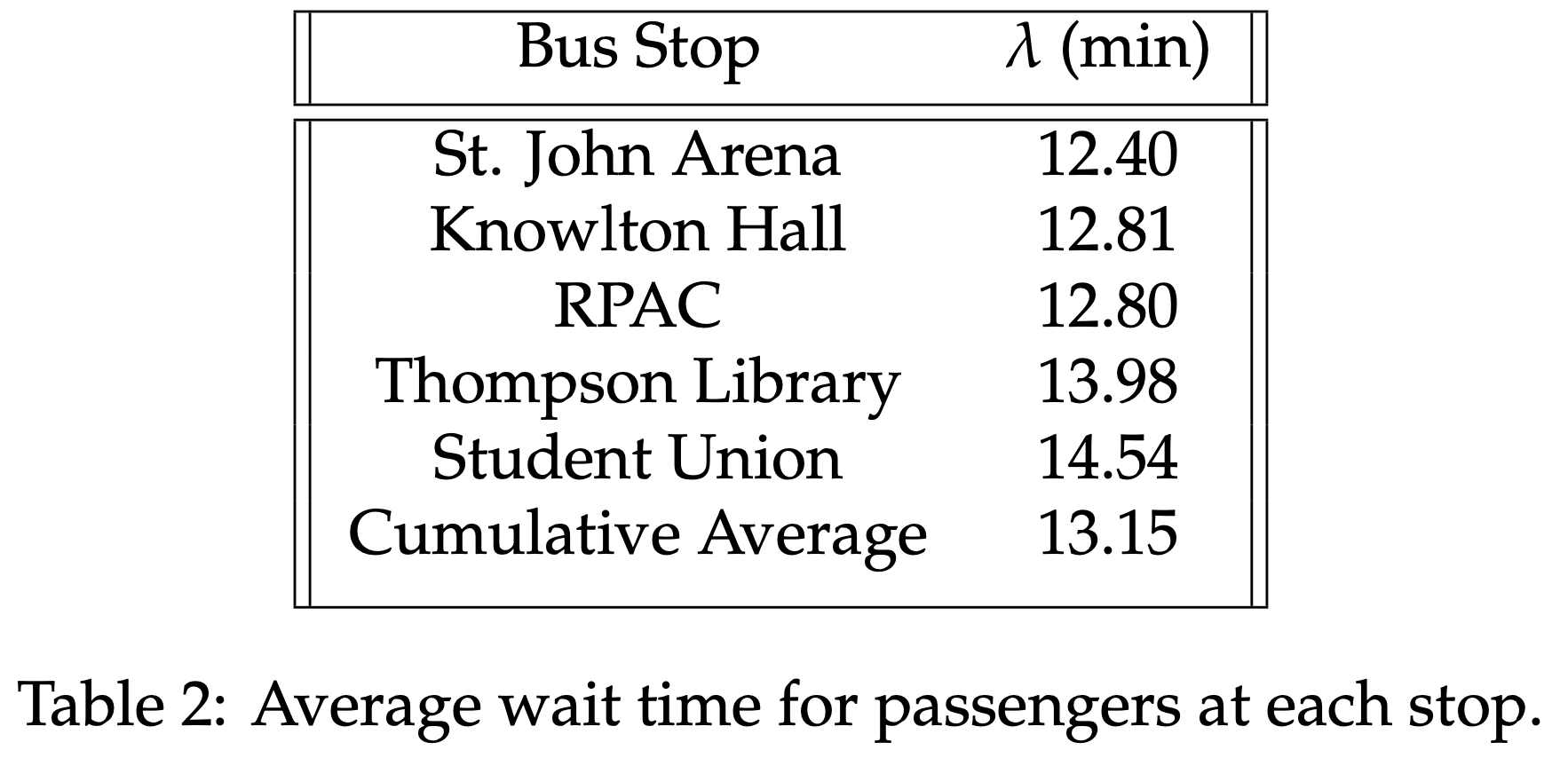
Time t is set to the duration of the experiment, which is 1 day in this instance. This parameter will be altered in Section III to view any potential distribution variation. Additionally, x represents each waiting time that is simulated, as opposed to expected. For instance, if the Student Union ends experimentation with waiting times of 2, 5, 9, 10, 11, 12, 12, 11, 1, 28, then each of those values will be utilized as values of x in the probability calculations. In other words, the calculation will be repeated for each waiting time x, while time (t) and expected waiting time (λ) remain unchanged for each stop. With these parameters, we can then apply the following theorem to calculate the expected probability of waiting times equating to x.

P(Arrivals = x) = e^(−λt(λt)) / (x!)

Applying this formula to a range of x values will provide us with a full picture of the distribution for each bus stop and the system overall. In this section, we layout the expected distribution of waiting times for each bus stop, along with the cumulative picture of all bus stops. These visualizations will then be used as a baseline for comparison to the simulated data in the ensuing section. The distributions are largely the same, as the only disparity between them lies in their respective I values. As such, one would expect the corresponding simulated waiting times to be independent in regard to bus stop. We will view these hypothetical distributions in the next section to offer a vivid examination of the empirical evidence, before concluding with our overall findings and future relevant areas of study.

Visualization

In this section, we initially view the simulated distribution of wait times. These graphs are pitted up against the theoretical output, seen above in part F of Section 2, to verify their validity. The section concludes with insight into additional circumstances that may lead to distribution changes, along with these altered distributions.

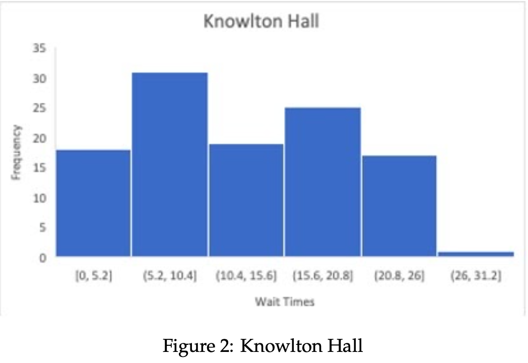
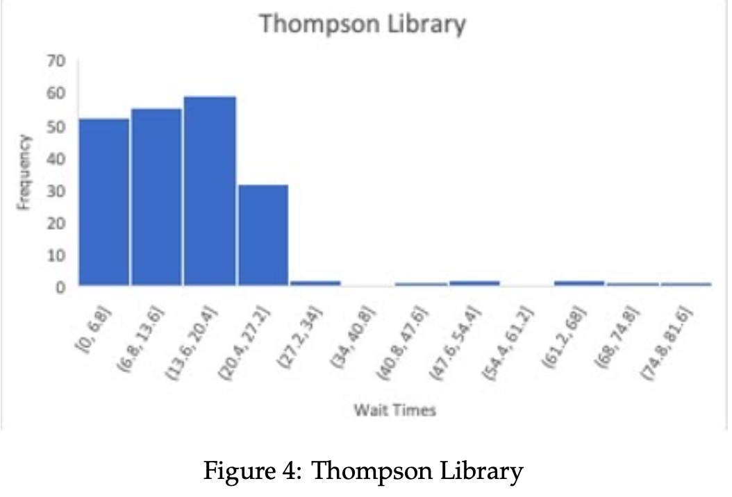
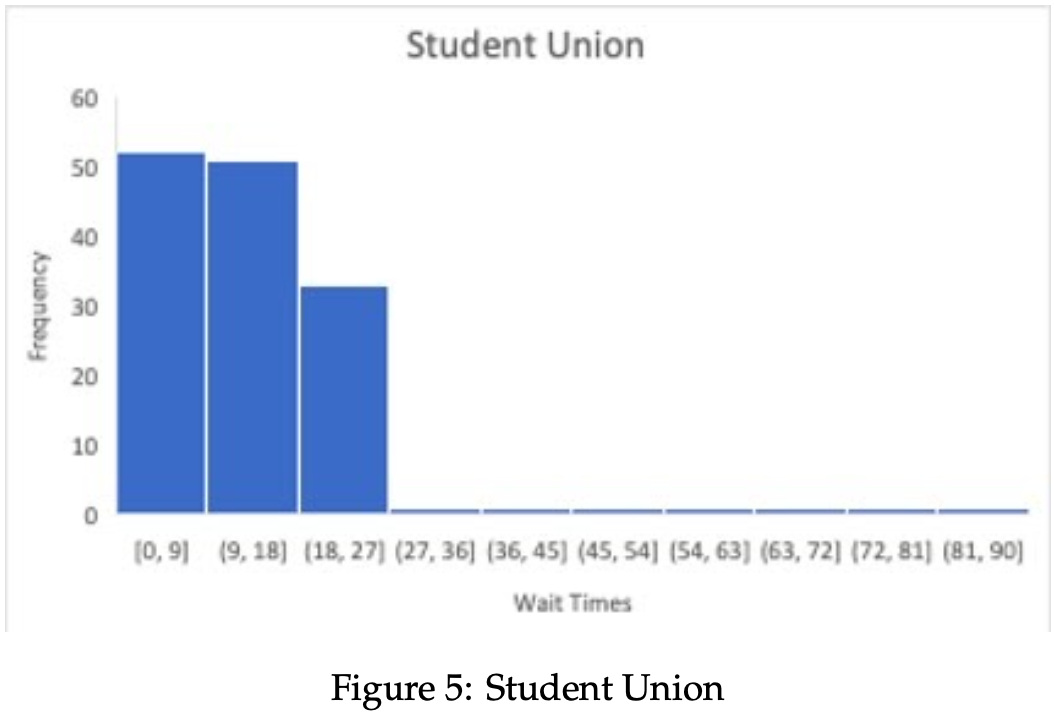
Empirical Wait Time Distribution The following data is retrieved from the "allTimes" ArrayList. The data structure "allTimes" tracks the wait times for passengers at each stop i, aˆ¦ , numStops, and outputs the data into an organized histogram. Below, the accumulated distributions for each bus stop, along with a cumulative result from all bus stops, are displayed. Wait times are shown in bins of minutes, with their respective frequencies listed along the vertical axis.

The data is acquired in a structurally randomized way, so the output is not meant to flawlessly replicate any specific distribution. In order to test its approximation to the Poisson Process, the empirical and theoretical values can be viewed simultaneously, which we provide in Table 3.
Expected and Simulated values differ significantly in certain wait time intervals, while the approxima- tion is more accurate in others. This occurs due to the nature of the experiment, as well as the theory behind a Poisson Process. To begin with, take a look at another table that illustrates the bus movement at the onset of the experiment.
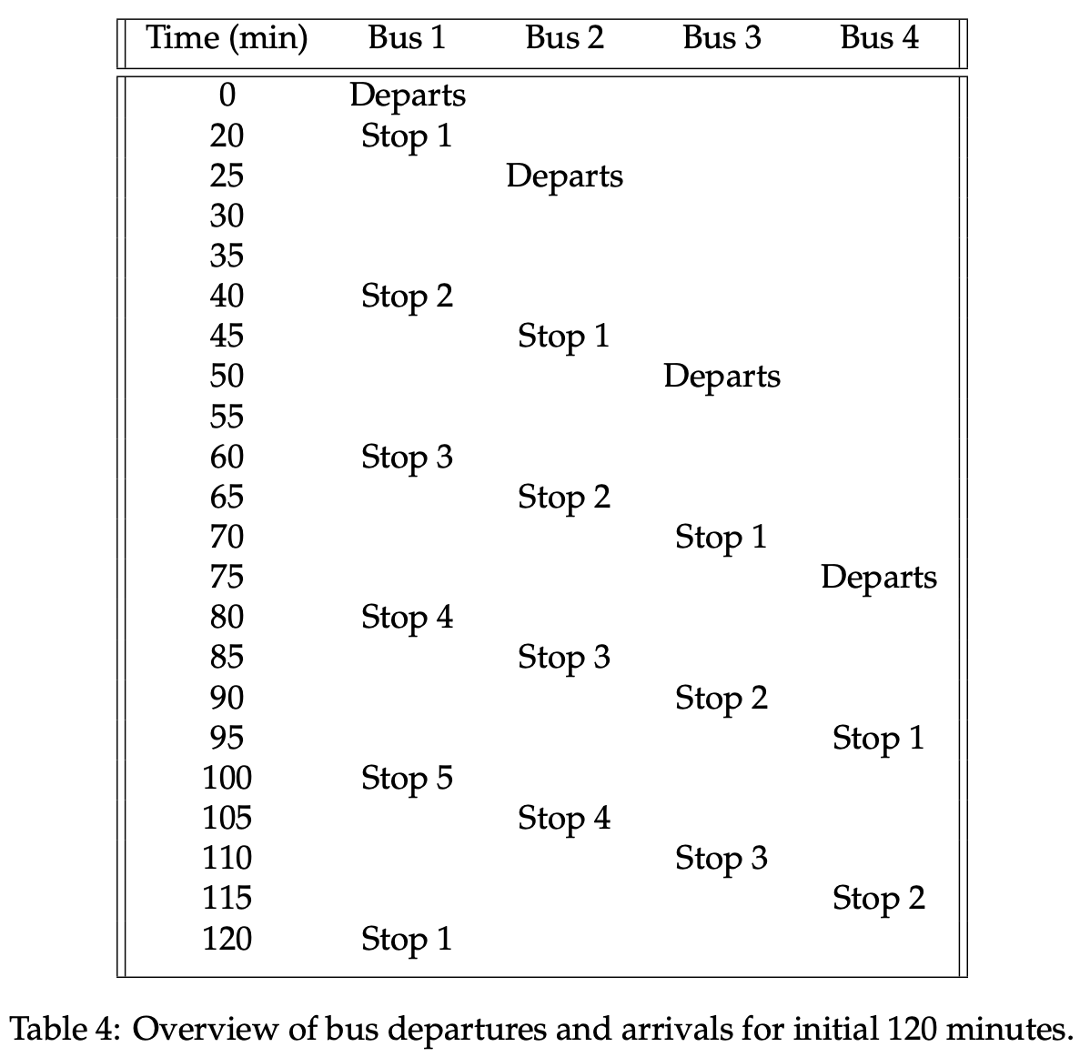
A bus will arrive at each stop i, . . . , numStops at a perpetual time interval of 25 minutes given the proposed simulation parameters. Since these arrival times are consistently dispersed, along with customer arrivals being randomized, then the probability of a passenger waiting anywhere from 1 to 25 minutes is the same throughout. The simulated data reflects this knowledge, as the only data is relatively uniform in frequency from [0, 25] minutes. Wait times beyond 25 minutes represent spillover from one bus to the next, and cannot be predicted as accurately as those in the bus stop arrival range. A proposed solution to this issue is discussed in the closing thoughts, as well as several alterations that can be made to the existing program structure.
Exploring Spillover Spillover has been mentioned multiple times in this study, and in this subsection we revisit it directly. The term is defined as one or more passengers being unable to board a bus due to it reaching capacity, causing the displaced passengers to wait for the next bus able to accommodate them. To test the impact of spillover on wait time distributions, we increased the arrival rates of passengers, while also lengthening the time it takes bus i to go from stop j → stop j + 1. These alterations are meant to represent a bus system that transports more of the general populace than the COTA system does in Columbus. Spillover is subject to the environment in which the bus system finds itself, and will vary depending on the specific input parameters. This segment portrays one possible implementation, and the results from All Bus Stops are displayed underneath.
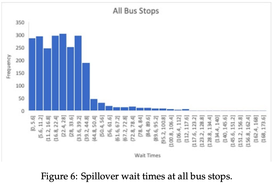
The distribution of times from [0, 25] remains largely unchanged. However, there is an evident increase in wait times in the interval immediately beyond 25 minutes and continuing until nearly 45 minutes elapse, equal to the span of (25, 45]. Longer wait times occur far less frequently, yet still more so than in the original data used earlier. Therefore, in more densely populated bus systems, it is fair to assert that the uniform distribution is extended beyond simply the bus distance interval. Additionally, an increasingly large proportion of wait times exist beyond one spillover bus arrival. In this case, the aforementioned longer wait times are greater than 50 minutes (2 * busDistanceInterval), and are far more prevalent than in the COTA replication.
Varying Simulation Duration We now revisit the idea of variable experiment lengths. The final distribution of times will hypothet- ically become more pronounced, regardless of which form it takes, as time t approaches infinity. In this subsection, we will increase the simulation length from 1 day to 1 week in an effort to verify the aforementioned hypothesis. The results are displayed below:
The results reflect what we have uncovered in shorter trials: the vast majority of wait times fall within the range of [0, busDistanceInterval], along with a few spillover cases as well. Since we looked at the distribution of more populated systems as well, it may prove beneficial to study that same circumstance over the course of 1 week to compare to the COTA replica.
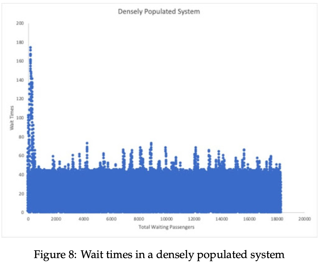
Over the course of nearly 15,000 more waiting passengers, the uniform distribution extended beyond simply [0, busDistanceInterval] to approximately 0-45 minutes. Additionally, the frequency of pas- sengers waiting for more than one bus at a time increases also. Interestingly, though, there appear to be fewer lengthy wait times when compared to the COTA population data. This could suggest that while passengers may have to wait longer on average, densely populated bus systems are more well equipped to handle sudden upticks in transit demand than their more sparsely traveled counterparts.

Concluding Remarks

This study introduces a hypothetical system of buses and bus stops, based on real life parallels. We then produce waiting times for a mass quantity of passengers before testing their corresponding distributions in relation to potential theoretical outcomes. We find that the empirical distribution trends toward uniformity as opposed to a Poisson Process. In systems in which consumer arrivals occur relatively infrequently, thus reducing emphasis on spillover, the wait times fall in the range of [0, busDistanceInterval]. Conversely, the trial that incorporated more waiting passengers into a system of increasingly spread out buses found the distribution frequencies spanned nearly twice the original COTA experiment. Hence, the resultant accumulation of wait times is impacted by spillover, while the distribution remains constant. This suggests that as long as bus route intervals remain consistent, the distribution of passenger wait times will be relatively uniform in nature.

Future research should take a look at a few variations of this project. This includes the distribution of buses along their respective routes, as well as the arrival rates of buses. Regarding bus allocation, this experiment commenced with one bus being dispersed at a time, until all buses were traversing routes. As a consequence, passengers arriving at the outermost routes see a spike in initial wait times. For example, assuming our parameters are in place, let Consumer A arrive at stop 4 at time t = 4 minutes. The first bus does not reach stop 4 until 80 minutes have elapsed, meaning Consumer A is forced to wait at least 76 minutes before boarding a bus. This may or may not be a desired scenario, depending on the bus system and city in consideration. Initially sending certain buses to later stops would more effectively distribute resources and service all bus stops equally during the first revolution. Alternatively, a bus system could simply direct potential passengers to wait until a certain operating time before waiting in line. The opening times of bus stops would then vary by the bus distance interval. Secondly, in order to more accurately replicate a Poisson Process, it may be prudent to provide randomness between bus arrival times. This would allow for more variation between waiting times and could potentially lead to a more centralized distribution. The randomized arrival times must be limited somewhat by the fact that bus systems are predicated on strict scheduling. However, exact arrival times do not occur, so a bus arriving several minutes early or late still provides meaningful data both theoretically and practically.

Sources

Baker, Samuel L. Queuing Theory I. p. 3-4, 2006.
Billey, Sara. Discrete Mathematical Modeling. University of Washington, p. 43-51, 2011.
Koehrsen, William. The Poisson Distribution and Poisson Process Explained. 20 Jan 2019.
Liu, Luyu and Miller, Harvey. "Does real-time Transit Information Reduce Waiting Time? An Empirical Analysis." Transportation Research Part A, p. 167-179, 6 July 2020.
VanderPlas, Jake. "The Waiting Time Paradox, or, Why is My Bus Always Late?" Pythonic Perambulations, 13 September 2018.